Transaction Attributes and Customer Valuation
Michael Braun
Cox School of Business
Southern Methodist University
David A. Schweidel
Goizueta Business School
Emory University
dschweidel@emory.edu
Eli Stein
Harvard College
Harvard University
estein@post.harvard.edu
Forthcoming in December 2015 issue of Journal of Marketing Research
Abstract
Dynamic customer targeting is a common task for marketers actively managing customer
relationships. Such efforts can be guided by insight into the return on investment from marketing
interventions, which can be derived as the increase in the present value of a customer’s expected
future transactions. Using the popular latent attrition framework, one could estimate this value
by manipulating the levels of a set of nonstationary covariates. We propose such a model that
incorporates transaction-specific attributes and maintains standard assumptions of unobserved
heterogeneity. We demonstrate how firms can approximate an upper bound on the appropriate
amount to invest in retaining a customer and demonstrate that this amount depends on customers’
past purchase activity, namely the recency and frequency of past customer purchases. Using
data from a B2B ser vice provider as our empirical application, we apply our model to estimate
the revenue lost by the service provider when it fails to deliver a customer’s requested level of
service. We also show that the lost revenue is larger than the corresponding expected gain from
exceeding a customer’s requested level of service. We discuss the implications of our findings
for marketers in terms of managing customer relationships.
Keywords:
services marketing, customer retention, probability models, marketing ROI, customer
value
1
According to IBM’s recent survey of chief marketing officers, 63% of respondents said that
return on investment (ROI) would be the most important measure of success in the next three to five
years (IBM Corporation 2011). Braun and Schweidel (2011) argue that marketing ROI should be
measured in terms of an expected change in the residual value of the customer base that occurs from a
marketing intervention. Latent attrition models, such as the the Pareto/NBD (Schmittlein, Morrison,
and Colombo 1987) and the BG/NBD (Fader, Hardie, and Lee 2005a), are useful for estimating
residual value, but they do not lend themselves easily to incorporating covariates that change from
transaction to transaction. In the marketing ROI domain, possible examples of these covariates
include attributes of the marketing mix, exogenous conditions at the time of the transaction (e.g.,
weather effects), or an investment in improved customer experiences.
The quality of customer information to which a firm has access, which encompasses being
both broad and up-to-date, has been found to moderate the profitability of customer prioritization
(Homburg, Droll, and Totzek 2008). Similarly, Mithas, Krishnan, and Fornell (2005) posit that the
value of customer relationship management tools lies in their ability to facilitate learning about
customers over the course of multiple interactions, the insights from which can then be used to target
customers dynamically with tailored offerings. Though some researchers have proposed methods of
incorporating both time-invariant and time-variant predictors into customer base analyses (Abe 2009;
Schweidel and Knox 2013), these models stop short of establishing the link between the effects
of transaction-specific attributes and forecasts of residual value. Thus, how to use information
about transaction attributes to assess the increased customer value stemming from marketing efforts
remains an open and important area of research.
In this paper, we propose a latent attrition model that integrates transaction attributes into a
probability model of customer retention and lifetime value. One application of this model (and the
one we use in our empirical analysis) is to evaluate the impact of a customer’s service experience on
customer retention. Consider the following scenario. A local business (i.e., the customer) contracts
with a service provider to meet a recurring business need, such as copywriting services. Based on
examples of the provider’s work, the customer has some expectation of the caliber and timeliness of
2
the work. If the provider delivers a top-notch experience, the customer may engage the provider
the next time he needs similar services. By increasing the retention probability for that customer,
all else being equal, the service experience delivered by the provider’s team may have generated
additional revenue in subsequent time periods. In contrast, if the provider falls short and delivers
a sub-par experience, the customer may be more likely to search for another provider when the
need for similar services arises in the future. When this happens, the future revenue stream from
the customer falls to zero. In this example, the attributes of a single customer-firm interaction
could affect the future revenue stream. The “transaction attribute” in this case is an indicator of the
customer’s service experience. More generally, transaction attributes may refer to some aspect of
the marketing mix, the employee who processed a customer’s transaction, or any information about
a customer’s transaction that the firm has collected.
While there is an intuitive relationship between transaction attributes and retention probabilities,
and hence customer value, extant empir ical research often fails to differentiate among transactions
other than with regard to the times at which the events occur. Models like the Pareto/NBD and
the BG/NBD rely on summary statistics of past transactional activity, namely the total number
of transactions (frequency) and the time of the most recent transaction (recency). However, by
aggregating the data to this level, information about other characteristics of each transaction is
lost. Take the case of two customers with the same number of transactions dur ing the last year,
and with their most recent transaction occurring on the same day. Ignoring attr ibutes of those
transactions, these two customers’ transaction histories, and the resulting predictions of residual
value, are identical. If a firm had access to additional information about the last customer-firm touch
point, the firm could have different beliefs of what each customer would do in the future. Failing to
meet stated and established standards of service, for example, may lead the firm to believe that a
customer is now at a g reater risk for churn, while exceeding these standards may lead to perceptions
that this risk is lower (Ho, Park, and Zhou 2006).
Exploiting information about the attributes of each transaction gives firms additional guidance for
managing customer relationships, compared to the information provided by frequency and recency
3
alone. The value of transaction attribute data comes from how that information affects the firm’s
decisions. We assess the effect of a particular transaction attribute in terms of the projected change
in discounted expected residual transactions (DERT, Fader, Hardie, and Lee 2005b; Fader, Hardie,
and Shang 2010). DERT is the present value of expected future transactions, taking into account
the probability that a customer may have already chur ned, or will churn in the future. Differences
in the transaction attributes will produce variation in DERT beyond that which is captured by
the recency and frequency of transactions. Attribute data can affect firm decisions in two ways.
First, ignoring attributes can lead to different estimates of DERT, which in turn may lead to a
suboptimal decisions based on bad information. Second, the “incremental DERT” that comes from
manipulating the transaction attributes (say, by increasing investment in retaining a specific customer
immediately before a transaction) can serve as an upper limit for such a marketing investment (Braun
and Schweidel 2011). For example, if a firm could estimate the effect of a marketing mix variable
on churn, the incremental DERT would be the difference between the forecast of DERT under the
marketing treatment, and a baseline DERT without it. To the best of our knowledge, our research is
the first to examine the value of information about transaction attributes in terms of the change in
expected future customer transactions.
In the next section, we provide a brief discussion of relevant literature in the customer base
analysis and service quality areas, the latter of which relates to the context of our empirical example.
We show how our research adds to the associated body of knowledge. Then, we describe the
model, in terms of a likelihood function, as well as derive both prior and posterior DERT that can
be expressed in either closed-form or as a summation. The subsequent empirical analysis, which
employs a dataset from a noncontractual service provider, illustrates a case in which including
transaction attribute data adds predictive power to the model. Finally, we show that incremental
DERT has a nonlinear and non-monotonic relationship with customer recency and frequency. The
patterns suggest that falling short of the requested service level has a smaller effect on retaining
customers who are either likely to have already chur ned, or who are highly unlikely to have churned,
compared to the effect on customers for whom there is more uncertainty in their active status.
4
1 Related Literature
Latent attrition models such as the Pareto/NBD and the BG/NBD are workhorse models of customer
base analysis (Schmittlein, Morrison, and Colombo 1987; Fader, Hardie, and Lee 2005a; Fader,
Hardie, and Lee 2005b). A notable limitation of this class of models is the difficulty of incorporating
information about attributes that accompany each customer-fir m interaction, such as marketing
actions that vary across transactions. Recognizing this gap in the literature, Ho, Park, and Zhou
(2006) propose incorporating customer satisfaction into the latent attrition framework. Their model
assumes that customer satisfaction affects the rate at which customers conduct transactions, and they
demonstrate how satisfaction can be allowed to impact the attrition process. Although Ho, Park, and
Zhou do consider information that is specific to the customer-firm interaction (i.e., satisfaction),
their model is analytic, as opposed to empirical. Nevertheless, they illustrate the importance of
incorporating customer satisfaction and, more broadly, customer-firm interaction information, into
estimates of customer value.
Another notable difference between the Ho, Park, and Zhou (2006) model and empirical latent
attrition models is that Ho, Park, and Zhou assume homogeneous purchase and attrition processes.
In addition to capturing variation across customers, models that allow for unobserved heterogeneity
let firms update their expectations of customer behavior as new data become available. These
posterior inferences are necessary both for valuing customers (Fader, Hardie, and Lee 2005a; Braun
and Schweidel 2011) and for assessing the impact of marketing efforts. Schweidel and Knox (2013)
illustrate this idea with a joint model of individuals’ donation activity and the direct marketing efforts
of a non-profit organization, accounting for the potentially non-random nature of marketing efforts.
In their example, the authors allow for direct marketing activity to affect the likelihood of donation
each month, the amount of a donation conditional on the donation occurring, and the likelihood
with which a donor becomes inactive. To account for unobserved heterogeneity, Schweidel and
Knox apply a latent class structure. While their model allows for marketing actions to impact
each of the processes that may affect customer value, they do not consider how an individual’s
transaction history may affect expectations of future activity. Moreover, they do not consider how
5
their framework could be adapted to estimate measures such as expectations of future purchases,
customer lifetime value, or residual value.
Like Schweidel and Knox (2013), Knox and van Oest (2014) also employ a latent class structure
to account for heterogeneity across customers in their investigation of the impact of customer
complaints on customer churn. They assess the impact of customer complaints and recovery by
the firm for two types of customers: a new customer and an established customer. The authors
demonstrate that the residual value of customers following a complaint varies with both the customers’
past purchase activity and past complaints. The authors distinguish between the effects of marketing
interventions on new and established customers, consistent with research that has investigated the
profitability of behavior-based marketing actions (Villas-Boas 1999; Pazgal and Soberman 2008;
Shin and Sudhir 2010). While extant work has documented the benefits of differentiating between
new and established customers, such work often does not seek to provide insight into how marketing
interventions may affect established customers with different transaction histor ies. We contribute to
this stream of research by developing a modeling framework that allows us to conduct a systematic
investigation into how customers’ recency and frequency of past transactions (Fader, Hardie, and
Lee 2005b) affects the incremental impact of marketing efforts, which can enable marketers to target
customers with increased precision.
Although there are many different attributes a transaction could possess, our empirical analysis
in Section 3 is in the domain of service quality. Several researchers have studied service quality and
its relationship to customer expectations. Boulding et al. (1993) find that a customer’s evaluation of
a service encounter is affected by his prior expectations of what will and should occur, as well as the
quality of service delivered on recent service encounters. In essence, will and should expectations
for a service encounter are a weighted average of prior expectations and the recently experienced
service. Boulding, Kalra, and Staelin (1999) further investigate the process by which expectations
are updated. In addition to affecting a customer’s cumulative opinion, the authors find that prior
beliefs also affect how experiences are viewed. As a result, prior expectations deliver a “double
whammy” to evaluations of quality. This suggests that service encounters are not all equal in
6
the eyes of consumers, as the way in which service encounters are viewed are affected by past
experiences. For example, the exact same level of quality might exceed expectations in a mid-range
family restaurant, but miss expectations in a fancy bistro. Yet, extant customer valuation models in
both non-contractual and contractual settings often assume that the “touch points” associated with
customer-firm interactions are equivalent to each other.
Rust et al. (1999) further investigate the role of customer expectations in perceptions of quality.
Rather than focusing on the average expectation across customers, the authors highlight the
importance of the distribution of customer expectations. They tackle a number of myths that had
been held with regard to the level of service that providers should deliver to their customers. In
contrast to the popularly held belief that firms must exceed expectations, the authors find evidence
that simply meeting customers’ expectations can result in a positive shift in preferences. They
also find that service encounters that are slightly below expectations may not affect customers’
preferences at all. Though provoking, the authors recognize that because they conducted their
investigation in a laboratory setting, and relied on self reports, there is a need for additional research.
In addition to the work that has been conducted on service quality, our research is also related
to work on customer satisfaction. Bolton (1998) investigates the impact of customer satisfaction
on the duration for which customers continue to subscribe to a contractual service. She finds that
reported customer satisfaction with the service, solicited prior to the decision of whether to remain
a subscriber or cancel service, is positively related to the duration for which a customer will retain
service. She also finds evidence that recent experiences with the service provider are weighed
differently depending on whether the experience was evaluated as positive or negative. To the best
of our knowledge, research on customer valuation has not incorporated this differential weighting of
customer experiences into estimates of customers’ future behavior.
7
2 Model
In this section we propose a general form of a latent attr ition model that incorporates transaction
attributes. To keep terminology consistent with the empirical example in Section 3, we say that the
customer of the firm places orders for jobs, and the firm fills those orders by completing the jobs.
Thus, orders and jobs always occur in a pair, and are indexed by
k
. We assume that these jobs are
completed the instant the order is placed, so we index calendar time for orders and jobs by
t
. Without
loss of generality, we define a unit of calendar time as one week. The service was introduced to the
marketplace at time
t =
0 and
T
is the week of the end of the observation period. Let
t
1
be the week
of the customer’s first order, let
x
be the number of orders between times
t
1
and
T
, including that
first order at
t
1
, and let
t
k
be the time of order
k
. Therefore,
t
x
is order time of the final, observed
job. For clarity, we are suppressing the customer-specific indices on
t
and
x
in the model exposition.
Our baseline model is a variant of the BG/NBD model for non-contractual customer base analysis
(Fader, Hardie, and Lee 2005a). Immediately before the customer places an initial order at time
t
1
,
he is in an active state. While active, the customer places orders according to a Poisson process with
rate
. After each job (including the first one), a customer may churn, resulting in that order being
his last. With probability
p
k
, the customer churns after the
k
th
job and transitions from the active
state to the inactive state. Upon doing so, we assume that the customer is lost for good and will
not place any more orders, ever. If the customer does not churn, then the time until the next order,
t
k+1
t
k
, is a realization of an exponential random variable with rate
. We never observe directly
when, or if, a customer churns, although if a customer places
x
orders, he must have survived
x
1
possible churn opportunities.
For a customer who places
x
orders between times
t
1
and
T
, the joint density of the
x
1
inter-order times is the product of
x
1 exponential densities. For this customer, there could not
have been any orders between times
t
x
and
T
. This “hiatus” could occur in one of two ways. One
possibility is that the customer may have churned after job
x
, with probability
p
x
. Alternatively,
the customer may have “survived” with probability 1
p
x
, but the time of the next order would be
sometime after
T
. Thus, conditional on surviving
x
jobs, the probability of not observing any more

8
jobs before time T is e
(Tt
x
)
. Hence, the conditional data likelihood for a single customer is
f (x, t
2:x
|, p
1:x
) =
x1
e
(t
x
t
1
)
2
6
6
6
6
4
x1
Y
k=1
1 p
k
3
7
7
7
7
5
f
p
x
+
1 p
x
e
(Tt
x
)
g
(1)
If
p
k
were time-invariant (i.e., the same for all
k
), Equation 1 would be the individual-level likelihood
in the BG/NBD
1
. To incorporate transaction-specific information, we allow
p
k
to vary across orders
in our model. We define the probability of becoming inactive by transitioning to the inactive state
immediately after job
k
as
p
k
=
1
e
✓q
k
and define
B
k
=
P
k
j=1
q
k
, where
q
k
is a non-negative
scalar value that can influence the probability that a customer transitions to the inactive state after
job
k
. If we restrict
q
k
=
1 for all
k
, then
p =
1
e
✓
, or alternatively,
✓ = log(
1
p)
. The
expression
q
k
, and hence
B
k
, could be a function of further parameters and observed data, such as
the transaction attributes. For example, we might give
q
k
a log-linear str ucture, where
log q
k
=
0
z
k
,
is a vector of homogeneous coefficients, and
z
k
is a vector of covariates that represents attributes
of transaction k. Substituting these definitions into Equation 1,
f (x, t
2:x
|, ✓, q
1:x
) =
x1
e
(t
x
t
1
)✓ B
x1
f
1 e
✓q
x
⇣
1 e
(Tt
x
)
⌘g
(2)
The expression of the likelihood in Equation 2 assumes that all customers place orders at the same
rate, and that all customers have the same baseline propensity to churn after each job. To incorporate
heterogeneity of latent characteristics into the model, we let
and
✓
vary across the population
according to gamma distributions, where
⇠ G
(r, a)
and
✓ ⇠ G
✓
(s, b)
. Integrating over these
latent parameters, we get the marginal likelihood:
L =
(r + x 1)
(r)
a
r
(a + t
x
t
1
)
r+x1
b
b + B
x1
!
s
2
6
6
6
6
4
1
b + B
x1
b + B
x
!
s
*
,
1
a + t
x
t
1
a + T t
1
!
r+x1
+
-
3
7
7
7
7
5
(3)
A detailed derivation of the marginal likelihood is in Equation 10 in Appendix A. Transforming
1As with the BG/NBD, in our model a high transaction rate suggests additional attrition opportunities.

9
a gamma-distributed random variable to yield a value between zero and one was discussed by
Grassia (1977). If
p
k
were constant across time, and varied across the population according to a
beta distribution, then the marginal likelihood would be the same as the BG/NBD. Griffiths and
Schafer (1981) show that Grassia’s method and a beta distribution are “practically identical,” and
that choice between them could be based “entirely on mathematical convenience.” Our approach
lets us estimate model parameters using standard maximum likelihood techniques even when the
attrition probability depends on transaction-specific covariates.
Certain design decisions allow us to maintain some degree of computational efficiency. We allow
for unobserved heterogeneity in
and
✓
by carefully choosing a parametric family of independent
mixing distributions. The
B
x
term is heterogeneous across observable characteristics that vary
across both individuals and time. Also, we allow for unobserved nonstationarity in some of the
parameters in B
x
(see Equations 8 and 9).2
2.1 Conditional expectations and DERT
Once a manager has parameter estimates in hand, he might be interested in the number of orders
that we might receive from a newly acquired customer during a period of
t
weeks. In Appendix A
we show that the prior expected value of this order count is
E[X (t)] =
1
X
k=1
b
b + B
k
!
s
H
B
✓
t
a + t
; k, r
◆
(4)
Therefore, the manager can estimate the expected number of orders by truncating this infinite series.
The function
H
B(x
;
a, b)
is regularized beta function, which also happens to be the cdf of a beta
distribution, with parameters a and b, evaluated at x.3.
One way to interpret the summation in Equation 4 is as the sum of the probabilities of ordering
2
Among the alternative specifications considered was one in which we allow for heterogeneity in
via a latent
class structure. The estimated probability of being in the first latent class was
p =
1, suggesting that the additional
model complexity is not warranted. We also estimated a model that allows
to vary with
z
k
. The Hessian in the
resulting model was singular, so the parameters could not be identified when covariates are assumed to impact both the
transaction rate and the attrition process simultaneously.
3A glossary of many of the functions we use in this paper is in Table 3 in Appendix A

10
k
jobs before time
t
, for all possible values of
k
. These jobs are hypothetical, so we need a model
for each
q
k
that comprises
B
k
, which is the cumulative sum of
q
1
, q
2
,...,q
k
. In general, one could
simulate multiple sequences of
q
k
from that model, truncated at a sufficiently large value of
k
, and
then average
E
[
X (t)
] across sequences. An alternative heuristic is to replace each
B
k
with its mean.
This approximation will be most accurate when the variance in
B
k
is very small, which, as we will
show later, is the case in our empirical application. This approximation is not needed to estimate the
model itself, but only to calculate the expected number of transaction without resorting to the use of
simulations.
A conceptually useful expression is the probability that a customer is still active at time T.
P (A) =
2
6
6
6
6
4
1
a + T t
1
a + t
x
t
1
!
r+x1
1
b + B
x
b + B
x1
!
s
!
3
7
7
7
7
5
1
(5)
The derivation for Equation 5 is in Appendix A.
A manager might also want to know how many orders he can expect from an existing customer,
during the next
t
⇤
periods, given an observed transaction history. In Appendix A, we show that this
posterior expected number of future transactions is
E
⇤
[X (t
⇤
)| x, t
x
] = P (A) ⇥
1
X
k=1
B
x
+ b
B
x
+ B
k
+ b
!
s
H
B
t
⇤
t
⇤
+ a + T t
1
; k, r + x 1
!
(6)
In Equation 6, the index of the summation
k
refers to the potential orders that are made after
time
T
. As discussed previously, we can either model
B
k
so that we may simulate future values of
B
k
explicitly, or substitute
E(B
k
)
as an approximation. The prior and posterior probability mass
functions for the number of orders (i.e., to express the probability of placing a particular number of
orders during some future number of weeks) are included in Appendix B, which is available as part
of the online supplement.
While it is useful to know the expected number of future orders, orders are placed at different
times. One order may be placed at time
T +
1, the next order may not be placed until a point in
time that is well into the future. Given the time value of money, orders that occur soon are more

11
valuable than orders that are placed later. Therefore, an appropriate metric for the expected number
of a customer’s future transactions should discount those transactions back to the present. The
value for discounted expected residual transactions (DERT) is proportional to a customer’s residual
lifetime value when the margin is constant (Fader, Hardie, and Shang 2010). Let
be a discount
factor that captures the time value of money, so a dollar earned
t
weeks from now is worth
t
today
(for notational simplicity, we reset the counter of
t
so
t =
0 at
T
, and we assume that payments are
made at the end of the week). The posterior estimate for the DERT of this customer is the sum of
discounted incremental expected orders.
DERT =
1
X
t=1
✓
E
⇤
[X (t)|x, t
x
, B
x
, T] E
⇤
[X (t 1)| x, t
x
, B
x
, T]
◆
t
= P (A)
1
X
k=1
B
x
+ b
B
x
+ B
k
+ b
!
s
⇥
1
X
t=1
t
"
H
B
t
a + T t
1
+ t
; k, r + x 1
!
H
B
t 1
a + T t
1
+ t 1
; k, r + x 1
!#
= (1 )P (A)
1
X
k=1
B
x
+ b
B
x
+ B
k
+ b
!
s
1
X
t=1
t
H
B
t
a + T t
1
+ t
; k, r + x 1
!
(7)
These future transactions depend on a number of different elements. The parameters
r
,
a
,
s
and
b
capture the distribution of order rates and baseline churn likelihoods across the population (e.g.,
for any randomly chosen member of the population,
E() = r/a
and
E(✓) = s/b
). Through
P (A)
,
customers with low
t
x
and high
x
might be more likely to have already become inactive, so there is
a low probability of these individuals conducting transactions in the future. Customers with high
x
and high t
x
are more likely to be alive, and to order often, so their DERT should be high.
Like all statistical models, this model is intended as a schematic of the actual data-generating
process. To give the model some useful parametric structure, we treat the latent attrition process as a
manifestation of a random variable. Though one can always propose more complicated versions of
a model, such as allowing for duration dependence in purchase times or contagion across customers
in their propensities to churn, we favor parsimony so as to avoid overparameterizing the model given
certain limitations in a typical transactional dataset.
12
3 Empirical Analysis
The context in which we study the role of quality on customers’ future transactions is that of an
online market for freelance writing services. The firm in question operates a website on which
customers can post orders for “jobs,” and from which writers can claim jobs to complete. The types
of jobs vary greatly. One example would be a 100-word description of a product that the customer,
an online retailer, is selling on her website. Another is a 500-word summary of what participants at
a conference might do for fun when exploring the host city. Orders include all of the information a
writer would need to complete the job: the topic area (e.g., sports, health), intended audience, word
count, and so forth. Customers are encouraged to be as specific as possible in their requirements,
as that makes it more likely the customer will be satisfied with the results. In our taxonomy, we
consider an order to be equivalent to the posting of a job.
Customers also choose a minimum rating, or grade, for the writers who are eligible to claim the
order. The firm maintains a bank of reviewers who screen and rate the writers who register with
the website. These reviewers are employed directly by the firm, and are considered to be experts
in evaluating prose (many have Masters of Arts degrees, or similar qualifications). Upon initial
application, a writer submits a writing sample, and a reviewer rates the writer as A, B, C or D. The
firm’s website provides examples of work from the different rating categories, so customers have a
general idea about the differences to expect across the different ratings. Ratings differ according to
objective criteria such as accuracy, grammar, style and vocabulary. A D-rated wr iter might produce
work with errors and simple sentence structure with no creative insight, while work from an A-level
writer will be of professional quality.
Customers pay, and writers earn, on a per-word basis, where the charge for each word depends
on the rating in the order. The firm claims a fixed percentage of this fee, plus a small (less than a
dollar) charge per order. Writers claim jobs from a list on a first-claim basis, so there is no bidding
involved. Wr iters may claim jobs that are rated below their own ratings (e.g., an A-rated writer
can choose a project from any level, but a B-rated writer cannot choose an A-rated order). In such
cases, writers are paid the lower per-word fee. The company has told us that it has not experienced
13
shortages of writers, with most job specifications being claimed within a day. Writers have another
day to complete the job, and nearly all jobs are completed within 24 hours of posting.
Sometime after the writer returns the completed job to the customer, the firm’s bank of reviewers
assigns each job a grade. Customers are not involved in this grading process, and neither customers
nor writers ever see the grade for a particular job. However, a writer’s rating can be adjusted
according to his grade history. This gives the writer an incentive to complete the job well; the grades
determine if the writer’s rating is adjusted up or down. The reviewers try to rate jobs as accurately
and objectively as possible, as a way to ensure that customers receive the quality they pay for, and to
reclassify writers as necessary. Writers can only be elevated to the A level manually, so the firm
classifies all A-rated and B-rated jobs together in an A/B class. Reviewers may also assign a grade
of E for completed jobs that do not meet even minimum standards.
3.1 Data summary
Our master dataset includes all completed jobs from the launch of the company in June 2008 to the
end of our observation period at the end of July 2011. We are restricting our analysis to customers
in either the United States or Canada whose first order takes place before the end of 2010, and to
jobs for which the language is English. This dataset contains information on 24,059 completed jobs
that were ordered by 3,048 distinct customers. For each job, we have identifiers for the customer
and writer, the day that the order was placed, some other details of the job specification. We also
have the requested rating of the job, as well as the grade the job received from the bank of reviewers.
Table 1 shows the number of jobs requested at each quality rating, and the quality grade of the work
that the writer delivered to the customer. By exploiting variation in the ratings, we can examine the
impact of quality level delivered (assessed objectively by the reviewer), relative to the level that was
requested by the customer, on customers’ future transactional activity.
All observed transactions for a particular customer occur from the day of a customer’s first order
(
t
1
), until the end of our observation period (
T
). Treating the time of initial trial as the beginning of
the customer relationship is consistent with prior research in customer base analysis (Schmittlein,

14
Post-hoc quality grade
A/B C D E Total
A 773 9 0 0 782
Requested B 8784 614 6 1 9405
Rating C 2050 5714 257 16 8037
D 1668 3270 814 83 5835
Total 13275 9607 1077 100 24059
Table 1: Number of jobs requested at each quality rating, and the quality grade of the work that the writer
delivered to the customer.
Morrison, and Colombo 1987; Fader and Hardie 2001; Fader, Hardie, and Lee 2005a). If a customer
places
x
orders during that observation period, his observed “frequency” is equal to
x/(T t
1
)
.A
customer’s “recency” is
t
x
, the week of the most recently observed order. Each day is represented as
1/7 of a week.
To control for the possibility that some of the firm’s earlier adopters might behave differently
than those customers whose first order came later, we divide the customer base into four cohorts
based on the week of the first order. The 588 customers who placed their first order during the first
33 weeks of our data are considered to be in the first cohort. The 568 customers who placed their
first order between weeks 33 and 66 are assigned to the second cohort. The 911 customers placing
their first orders between weeks 66 and 99 are assigned to the third cohort, and the 981 customers
placing their first orders between weeks 99 and 130 are assigned to the fourth cohort.
3.2 Model estimation
In this example, the transaction attr ibutes represent the requested and delivered quality of the jobs.
Although there are many functional forms that we could choose, we consider models of the form
log q
k
=
0
z
k
, where
z
k
is a vector of job-specific covariates and
is a vector of coefficients. Effects
that increase q
k
increase the probability of churn.
The elements of z
k
include the following:
- z
first
: a indicator of the customer’s first job;
- z
coh2
, z
coh3
, z
coh4
: indicators for time-invariant cohort effects;
15
- z
Ak
, z
Ck
, z
Dk
: indicators for the requested quality level of job k;
- z
Lk
,
z
Hk
: indicators for whether job
k
was lower (L) or higher (H) than the requested service
level; and
- z
LD
, z
HD
, z
LC
: interactions among requested and delivered quality ratings;
All coefficients, except those on
z
Lk
and
z
Hk
, are stationary. The coefficients
Lk
and
Hk
represent the effect on the churn probability from missing or exceeding the specifications of job
k
.
These effects can change from job to job, according to the customer’s recent experience. To capture
how these sensitivities change, we define a set of six
⌘
parameters that affect
Lk
and
Hk
in the
following ways:
L,k+1
=
Lk
+ ⌘
L
+ ⌘
LL
z
Lk
+ ⌘
HL
z
Hk
(8)
H,k+1
=
Hk
+ ⌘
H
+ ⌘
LH
z
Lk
+ ⌘
HH
z
Hk
(9)
The coefficient
Lk
changes by
⌘
L
regardless of the rating given to job
k
, capturing a drift in
customers’ sensitivity to receiving a lower-than-requested service level. The terms
⌘
LL
and
⌘
HL
capture the extent to which customers’ sensitivity to receiving a lower-than-requested service level
on job
k +
1 is affected by receiving a lower (
⌘
LL
) or higher (
⌘
HL
) level of service than was requested
for job
k
. The coefficient
Hk
evolves in a similar manner. By allowing
to be dynamic in this
way, we allow for customers’ responses to service quality to be affected by a customer’s experience
(Bolton 1998). For example, if
⌘
LL
were positive, then after having a bad experience with the firm,
a customer would be even more sensitive to subsequent bad experiences.
To assess the role of ser vice quality on churn propensities, we tested three variants of the model.
Model 3 is the full model as described. Model 1 is a “baseline” model that ignores all service quality
effects. Model 2 is similar to Model 3, with all of the insignificant ⌘ parameters removed.
Table 2 contains descriptions of the model parameters, along with maximum likelihood estimates
and standard errors. The subscripts for the elements of
in the table correspond to those of
z
. The
most interesting estimates are those on
L1
and
⌘
LL
, which are both positive. This result suggests

16
Model 1 Model 2 Model 3 Description
est se est se est se
r 0.90 0.04 0.90 0.04 0.90 0.04 shape parameter on
a 0.77 0.04 0.77 0.04 0.77 0.04 scale parameter on
s 1.09 0.07 1.08 0.07 1.10 0.07 shape parameter on ✓
b 1.13 0.19 1.14 0.19 1.17 0.20 scale parameter on ✓
first
-0.22 0.07 -0.22 0.07 -0.21 0.07 effect of customer’s first job
coh2
-1.15 0.11 -1.16 0.11 -1.15 0.11 fixed effect for cohort 2
coh3
-1.00 0.10 -1.01 0.11 -1.00 0.11 fixed effect for cohort 3
coh4
-0.81 0.11 -0.81 0.11 -0.80 0.11 fixed effect for cohort 4
A
0.88 0.11 0.89 0.11 0.89 0.11 effect for requested quality level A
C
-0.30 0.06 -0.27 0.07 -0.27 0.07 effect for requested quality level C
D
-0.51 0.08 -0.36 0.15 -0.37 0.15 effect for requested quality level D
L1
0.19 0.13 0.21 0.14 effect for rating being “lower” than requested
H 1
0.01 0.09 0.01 0.10 effect for rating being “higher” than requested
LD
0.21 0.36 0.24 0.38 interaction effect between “lower” and requested level D
HD
-0.18 0.17 -0.15 0.17 interaction effect between “higher” and requested level D
LC
-0.53 0.26 -0.52 0.26 interaction effect between “higher” and requested level C
⌘
L
-0.01 0.01 evolution parameter on
L
⌘
H
0.00 0.01 evolution parameter on
H
⌘
LL
0.18 0.12 0.29 0.21 evolution parameter on
L
after a “lower” rating
⌘
LH
0.05 0.13 evolution parameter on
H
after a “lower” rating
⌘
HL
0.01 0.04 evolution parameter on
L
after a “higher” rating
⌘
HH
-0.01 0.02 evolution parameter on
H
after a “higher” rating
Table 2: Parameter estimates
that, as expected, missing the requested level of service for the first job increases the probability of
churn. It also suggests that the magnitude of that effect will be larger for the next job with a missed
service level. Thus, the churn probabilities increase across jobs when customers repeatedly receive
lower-than-requested service.
We also see that
H1
, and the associated
⌘
parameters, are not significantly different from zero.
This asymmetry in the effect of service quality on customers’ tendency to churn is consistent with
losses looming larger than gains (Kahneman and Tversky 1979; Hardie, Johnson, and Fader 1993).
Our findings are also in line with prior research by Bolton (1998), who found that perceived losses
adversely impact the duration of a customer’s relationship in a contractual setting while perceived
gains did not have a significant impact on the duration of the relationship.
17
3.3 Model assessment
We compare the performance of the three model specifications using a series of assessments. A
likelihood ratio test suggests a weak preference for Model 2 over Model 1 (
2
6
=
11
.
0
, p = .
088);
we cannot infer a preference for Model 3 over Model 2 (
2
5
=
1
.
29
, p = .
936), or for Model 3
over Model 1 (
2
9
=
10
.
1
, p = .
342). One shortcoming of relying only on the likelihood ratio test,
however, is that it does not consider the extent to which the incorporation of transaction attributes
improves forecasting performance. Thus, in addition to the likelihood ratio test, we compare model
performance using two additional measures of fit.
We calculated the mean absolute percentage error (MAPE) associated with the models’ prediction
of the weekly number of repeat orders made by customers in our sample and the root mean squared
error (RMSE) for the models’ predictions of the distribution of the number of orders made by the
sample. We find that the MAPE is similar across model specifications, with Models 2 and 3 having
slightly lower errors compared to Model 1. In terms of the RMSE, we again find evidence to suggest
that the transaction attributes contribute to model fit. Models 2 and 3 have lower RMSEs compared
to Model 1 for the data used to estimate the model during the calibration and forecasting periods.
Using a holdout sample for cross-validation reveals that, while Model 2 has a lower RMSE than
Model 1, Model 3 has a higher RMSE during the forecasting period which would suggest that the
model is overparameter ized.
Details of these posterior predictive tests are in Appendix C, which as available as part of the
online supplement. Taken together with the likelihood ratio test, we believe that the posterior
predictive tests provide evidence that transaction attributes improve model performance and
contribute to forecasting accuracy. Based on these analyses, we focus on the results using Model 2
for the remainder of our discussion.
To provide a better sense for how well the proposed model captures customers’ observed behavior,
the panels in Figure 1 illustrate model fit at the aggregate level. Figure 1a plots the cumulative and
incremental number of weekly orders, for both in-sample and holdout populations. The vertical
lines at Week 130 divide the calibration and forecast time periods. We used only data to the left of
18
the lines for estimating the model parameters, and we included only those customers whose initial
order was before Week 130. Model 2 does well in tracking the number of orders from week to week.
In Figure 1b, we compare the histogram of pre-customer order counts with the distribution of counts
from Model 2 predicts. Again, Model 2 appears to fit rather well.
At the level of an individual customer, one managerially relevant test statistic is the probability
that a customer will place an order sometime in the future. While the probability of being active,
P (A)
, is a commonly used construct in customer base analysis, we cannot use it as a model checking
tool because we cannot observe the customer’s activity state directly. Instead, the appropriate metr ic
is
P
⇤
(
0
) = P(X
⇤
(t
⇤
) =
0
|x, t
x
, ·)
, the posterior probability that a customer will place no orders
during a forecast period. We test how well Model 2 predicts which customers will order during the
forecast period using a calibration plot. First, we assign each customer to one of 15 “bins”, according
to the customer’s posterior
P
⇤
(
0
)
. A customer is assigned to bin
i
if
(i
1
)/
15
< P
⇤
(
0
) i/
15
for
i =
1
...
15. Next, we compute the observed proportion of customers in each bin who do
not place an order during the forecast period. We consider the model to be well-calibrated if
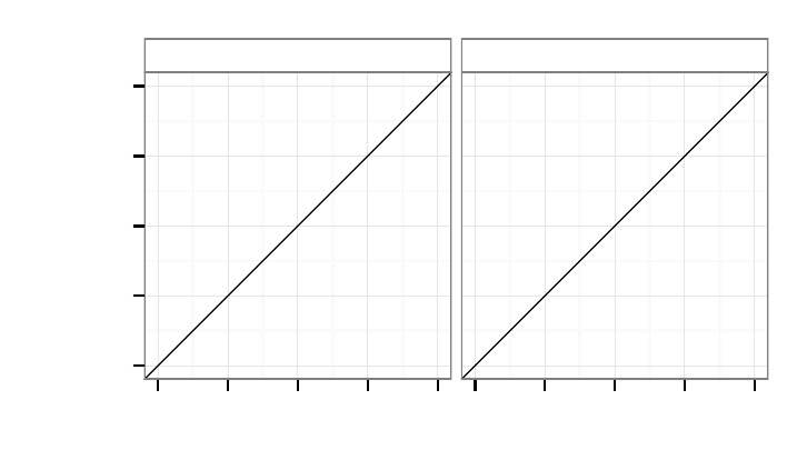
the predicted probabilities and observed proportions are aligned. Figure 2 confirms that they are.
Each dot represents the membership of the bin. The
x
-coordinate is the midpoint of the bin, and
the
y
-coordinate is the observed incidence of “no orders” for the members of that bin. “Perfect”
calibration would have occurred if all of the dots fell exactly on the 45° line. Of course, we expect
some random variation around this line, so we can still be confident that Model 2 forecasts the
incidence of future orders, at the customer level, quite well.
3.4 Forecasting quality data
In Section 2.1 we discussed the need to model the sequences of covariates for the purpose of
estimating conditional expectations and DERT rather than simply plugging in a fixed value. The
specifics of such a model depend on the context. For this dataset, there are two sources of variation
in the covariates: the ser vice level that a customer requested and the level that was delivered. For the
“requested” model, we assume that each customer has a latent, stationary probability of placing A, B,

19
Calibration Sample
Holdout Sample
0
5000
10000
15000
0.0
0.1
0.2
0.3
0.4
0.5
Cum. Repeat Orders
Incremental Orders / Trier
0 50 100 150 0 50 100 150
Week Since Launch (Forecast period begins Week 130)
Orders
model
Observed
Model 2
(a) Weekly incremental repeat orders per previously acquired customer. The vertical line is at Week 130, the
end of the calibration period and the start of the forecast period.
Calibration Sample
Holdout Sample
0
200
400
600
0
500
1000
1500
2000
Calibration Period
Forecast Period
0 1 2 3 4 5 6 7 8 9 10111213+ 0 1 2 3 4 5 6 7 8 9 10111213+
Number of Orders
Number of Clients
model
Observed
Model 2
(b) Observed and predicted histograms of orders.
Figure 1: Fit and forecast assessment for Model 2.
20
Calibration Sample
Holdout Sample
●
●
●
●
●
●
●
●
●
●
●
●
●
●
●
●
●
●
●
●
●
●
●
●
●
●
●
●
●
●
0.00
0.25
0.50
0.75
1.00
0.00 0.25 0.50 0.75 1.000.00 0.25 0.50 0.75 1.00
Probability of no orders during forecast period
Observed proportion of clients with
no orders during forecast period
Figure 2: Predicted vs observed probability of a particular customer making no orders during the forecast
period.
C or D-rated orders. This probability vector is heterogeneous and varies across customers according
to a Dirichlet distribution, allowing some customers to always choose the same rating, while other
customers vary more in their choices. Under the further assumption of a zero-order choice process,
we can infer the likelihood of a particular order pattern by using the maximum likelihood estimates
of a Dirichlet-multinomial mixture model.
The Dirichlet-multinomial parameters for this dataset are .04, .26, .22 and .12 for ordered
ratings A, B, C and D, respectively. These low values (all less than one) suggest high polarization
in the Dirichlet mixing distribution; even though there may be variation across customers, a
single customer is likely to place orders for the same level of quality across the jobs he orders.
To simulate hypothetical orders, we sample a probability vector from each customer’s posterior
Dirichlet distr ibution. Since most customers order at the same rating level every time, these posterior
probabilities are even more concentrated on a single quality level compared to the choice probabilities
of the prior distribution. We then use the empirical distribution of the job grades for each rating
level to get the service level delivered for each simulated job. In general, we find that there is little
variation in B
k
across simulated sequences of z
k
.
21
4 How Transactional Patterns Affect DERT and Incremental
DERT
Using the parameter estimates of Model 2, we can examine how infor mation from transaction
attributes affects expectations of the future transactional activity of heterogeneous customers.
Specifically, we examine how falling short of the expected level of service affects DERT, for
customers with different frequency (
x
) and recency (
t
x
) data. Figure 3 plots the contours that connect
the same levels of DERT at
T =
130 for hypothetical customers who placed the first order at time
t
1
=
1, and who requested quality grades B, C or D for the most recent order. For each of requested
service levels, we consider delivered service levels that are lower than, or the same as, what was
requested for that most recent order. We assume that the level of service delivered was the same as
what was requested for all other orders placed by the customer. These iso-value cur ves are similar
in spirit to those introduced by Fader, Hardie, and Lee (2005b) for the Pareto/NBD model. Since
DERT is a posterior expectation based affected by the likelihood that a customer remains active,
as anticipated, we see “backward-bending” contours (Fader, Hardie, and Lee 2005b). When the
number of orders is large and the most recent order was in the distant past, it is more likely that the
customer has already become inactive than if the x
th
order was made more recently.
The iso-DERT curves in Figure 3 reveal the relationship between customers’ transaction histories
and expected future activity, but they do not show the incremental effect of missing the requested
service level. To assess the incremental impact of deviations in the level of service on expected
future transactions, we calculate the difference in DERT between what we would expect when the
most recent job is rated at the same level of service the customer ordered and what we would expect
if the level of service delivered was lower. We refer to this difference as “incremental DERT.” This
metric offers a long-term assessment of the marketing investment’s impact, and forms an upper
bound on the amount the fir m should invest. In transactions for which incremental DERT is small, it
may not be worth the firm’s effort to monitor and evaluate the service encounters. Those transactions
for which the incremental DERT is large, however, may warrant additional resources to ensure the

22
Rating Lower
Rating as Ordered
10
20
30
10
20
30
10
20
30
Job Ordered D
Job Ordered C
Job Ordered B
90 100 110 120 130 90 100 110 120 130
Week of last order
Number of orders during calibration period
1
2
3
4
5
level
Figure 3: DERT iso-value curves for hypothetical customers whose first order came at
t
1
=
1. The panels
condition on the ordered job quality, and whether the last job was rated lower or the same than what was
ordered. The
x
axis of each panel is the week number of the most recent order (
T =
130), and the
y
axis is the
number of observed orders.

23
appropriate level of service is delivered. In our empir ical context, incremental DERT can be viewed
as the penalty associated with delivering a level of service lower than what a customer requested.
The expected cost of missing a requested service level for a brand new customer is the incremental
DERT when
x =
1 and
t
1
= t
x
= T
. That is, immediately after the first job is ordered and a
new customer comes under observation, incremental DERT is the number of discounted future
transactions that we expect to be lost if the delivered service level were below what was requested.
For this par ticular dataset, the percentage change is 2.9% for new customers who ordered a B-level
job, 2.5% for a C-level job, and 2.2% for a D-level job. For existing customers, incremental DERT
depends crucially on how many orders the customer has placed and how long ago his last order
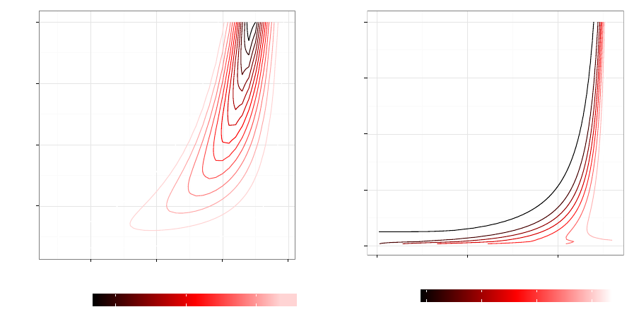
was made. Figure 4 shows this relationship in the form of “iso-incremental DERT” curves for a
customer who has requested a service level of B, in both absolute and percentage terms, for
t
1
=
1
and
T =
130. The levels of these curves represent the incremental DERT, evaluated at varying levels
of frequency and recency. The darker contours represent differences that are more negative, for
which the mismatch in service levels has more of an effect.4
In absolute terms, at a given level of frequency, falling short of the requested service level
appears to have the greatest effect when recency is neither too high nor too low. Take the case of a
customer who has conducted a given number of transactions. If the last transaction was conducted
recently, it is likely that the customer is still active. Regardless of whether the service delivered was
at or below the level requested, the recency of the transaction leads us to estimate a high DERT
for that customer. Alternatively, if the order were placed at a time in the distant past, the customer
is more likely to have already defected, regardless of the service quality level, so we estimate a
low DERT. In both of these cases, the difference in DERT between the case in which the service
delivered matches what was requested and the case in which it is below that which was requested
will be small compared to the incremental DERT for a customer with moderate recency. For those
customers, there is more uncertainty about whether the customer is still active. Small differences in
attrition probabilities will yield more substantial decreases in DERT when the requested service
4
We observe a similar pattern as depicted in Figure 4 for jobs that exceed the order specifications, except with
positive differences in DERT. However, for this dataset, the magnitude of the effect is very small.
24
25
50
75
100
100 110 120 130
Week of last order
Number of orders during calibration period
−0.06 −0.04 −0.02
Incremental
DERT
(a) Absolute difference
0
25
50
75
100
0 50 100
Week of last order
Number of orders during calibration period
−8% −6% −4% −2%
Percent
Incremental
DERT
(b) Percent difference
Figure 4: Iso-incremental DERT curves when missing the requested ser vice level. Observed recency is on the
x-axis and frequency is on the y-axis. Each curve connects points for which the incremental DERT is the
same.
level is missed. We see that the range of incremental DERT is the widest at low or moderate order
frequencies.
Figure 4b illustrates the DERT contours in percentage terms. As shown in Figure 4a, for a given
number of orders
x
, there are two values
t
x
that correspond to the same absolute difference in DERT.
As DERT increases with recency for a given value of
x
(as shown in Figure 3), incremental DERT
on a percentage basis will be smaller at higher values of recency.
Figure 4 demonstrates that the expected difference in a customer’s remaining value between
meeting and falling short of the requested service level depends on both the recency and frequency
of the customer’s transactions. When the goal of CRM is to identify those customers for whom
targeted marketing actions generate the greatest financial impact, our findings should caution against
scoring customers solely on popular measures like P(Alive) or CLV. While the most recent and
frequently transacting customers are likely to be the most valuable, the effect of transaction attributes
is not much different from customers who last purchased a long time ago.
To provide another perspective on customers’ remaining value, Figure 5 shows incremental
25
DERT (absolute in Figure 5a, and percent in Figure 5b) as a function of frequency, for select
values of recency. That is, each curve corresponds to a vertical slice of either Figure 4a or 4b.
For transaction histories with lower recency (e.g.,
t
x
=
85 and
t
x
=
100), we observe an initial
increase in the magnitude of the incremental DERT (in absolute terms) as the number of orders
increases. But, with a very large number of orders, the magnitude of incremental DERT decreases
and approaches zero. This patter n reveals the interplay of two factors. First, the large number of
orders is indicative of a high transaction rate (
). For these customers, missing the requested service
level puts a lucrative revenue stream at risk. But, with a large number of orders, the low recency of
the last order suggests that the customer may have already become inactive. Given that the increased
likelihood that the customer has already lapsed, the increased cost associated with missing the
requested service level is lower, resulting in the reduced magnitude of incremental DERT. At the
highest level of recency (
t
x
=
130), the customer is known to be still active, and DERT increases
with the number of orders. We thus observe that the magnitude of incremental DERT increases with
frequency, but at a much slower rate.
Figure 5b presents a similar analysis in percentage terms. At the highest level of recency
(
t
x
=
130), when the customer has just conducted a transaction and is known to still be active, DERT
increases with frequency. Therefore, incremental DERT, while relatively flat in absolute terms,
falls when expressed as a percentage of DERT. For the remaining three levels of recency, higher
transaction frequency ultimately results in a higher magnitude of incremental DERT as a percentage.
As the number of transactions increases along these three curves, so too does the likelihood that these
customers have already become inactive, thereby driving down DERT. With incremental DERT (in
absolute terms) being compared to a smaller base, the incremental DERT increases as a percentage.
Prior research has suggested that the value of CRM tools lies in their ability to facilitate learning
about customers (Mithas, Krishnan, and Fornell 2005), and that this value is limited based on the
quality of infor mation the firm has available about its customers (Homburg, Droll, and Totzek 2008).
Our findings reveal that differences in customer value that are associated with variation in transaction
attributes (e.g., the level of service delivered on a transaction) depend on customers’ past transaction

26
−0.020
−0.015
−0.010
−0.005
0.000
0 25 50 75 100
Number of Orders
Incremental DERT
Week of
last order
85 100
115 130
(a) Absolute difference
−8%
−6%
−4%
−2%
0%
0 25 50 75 100
Number of Orders
Percentage Incremental DERT
Week of
last order
85 100
115 130
(b) Percent difference
Figure 5: Absolute and percent incremental DERT as a function of frequency, for different levels of recency.
activity. If a customer is more obviously active or inactive deviations from the requested service
level provide little information on the customer’s DERT. It is when there is increased uncertainty as
to whether a customer is active or inactive that the level of service delivered relative to that which
was requested allows us to learn more about a customer’s DERT. To the best of our knowledge, our
research is the first to explore the value of transaction attributes using the latent attrition models
frequently employed in customer base analysis and customer valuation, and how past activity affects
the differences in customer value associated with transaction attributes.
5 Discussion
We present a flexible latent attrition model that incorporates transaction attributes in customer base
analysis, and descr ibe an empirical application that defines those attributes as indicators for relative
service quality. The model allows us to derive “incremental DERT,” a metric of the discounted
expected return on changes in those attributes. For transactions that are about to happen immediately,
incremental DERT can serve as an upper bound on the amount a firm should invest to change one
27
of those attributes. We also describe patterns in the relationship between incremental DERT and
the recency/frequency profile of the customer. Understanding these patterns and quantifying the
effects allow a manager to more accurately estimate DERT for all members of the customer base.
Model parameters can be estimated using standard maximum likelihood methods and DERT can be
computed as a truncated summation.
As firms use customer base analysis and customer valuation models to score and rank customers
according to the value they hold for a firm (Wuebben and von Wangenheim 2008), managers should
be interested in tracking and compiling transaction attributes that may be informative of customers’
future value. Acquiring such information, however, often entails a cost. For example, firms may
incur costs to monitor their salesforce to ensure compliance with required activities (John and
Weitz 1989). A simple heuristic to identify those transactions in which firms should be willing to
invest more in monitoring could be customers’ purchase frequency. After all, such customers are
likely to be among the most valuable customers to a firm. Our results, however, suggest that for such
customers, the difference in discounted long-term value to the firm between meeting and falling
short of the requested service level (reflected by incremental DERT) is low for those customers. For
customers who have not conducted as many transactions, our estimates of their value to the firm
are more sensitive to information on the level of service delivered. It is these customers for whom
estimates of long-term value are most subject to change if the level of service in a transaction comes
up short of specifications.
In our empirical context, we see that the magnitude of the effect of missing specified levels of
service is larger than exceeding specified levels. This is consistent with the idea of losses looming
larger than gains. While extant research has questioned the wisdom of trying to delight customers
by exceeding their expectations, due to the possibility of raising customers’ future expectations
(Rust and Oliver 2000), our analysis suggests that coming up short of the service customers have
requested poses a greater risk to a customer’s continued relationship with the firm and the firm’s
ability to capture the corresponding revenue stream.
Using our framework as a foundation, there are a number of promising directions with which
28
research could continue. While we focus our attention on customer retention and the value of
existing customers, a similar modeling approach could be employed to jointly investigate customer
acquisition and retention (Schweidel, Fader, and Bradlow 2008; Musalem and Joshi 2009). Doing
so could provide firms with guidance for how to balance marketing expenditures across the two
activities (Reinartz, Thomas, and Kumar 2005). Another area to explore is the effect of strategic
investments in service quality, a practice that the firm that supplied our data did not employ. While it
may be costly for a firm to invest in improving service encounters and monitoring these encounters
for all customers, the firm may have resources to focus on select customers. The firm could use
incremental DERT as a criterion for selecting those target customers. If the costs of delivering better
than expected service experiences are the same across customers, such an allocation rule would be
equivalent to putting your money where it will deliver the most “bang for the buck.” These actions
would be consistent with the management principle of “return on quality.” (Rust, Zahorik, and
Keiningham 1995). In many cases, we would need to account for the firm’s actions when estimating
the effect on retention probabilities (Manchanda, Rossi, and Chintagunta 2004; Schweidel and
Knox 2013). To alleviate such concerns, one might choose to proceed in this research area with a
carefully designed field experiment.
Another area for future research would be to develop further means of accounting for variation in
the effect of customer-firm touch points on future customer behavior. While we rely on observable
transaction attributes (i.e., the requested and evaluated service levels) as a means of evaluating
the level of service, future work may explore if such a measure could be inferred with additional
information about the transaction. For example, in our empirical context, if the transaction data
indicated the writer who completed each job, the firm may be able to evaluate the “quality” of each
writer based on the effect they have on customer churn. Another example of a firm that offers a
marketplace is eBay, which connects buyers and sellers. Evaluating sellers based on the churn of
buyers who have recently interacted with them may provide an indication of which sellers should be
rewarded versus which sellers are potentially costing the firm business.
A cost of conducting such an analysis is the detail in the data that must be collected. While

29
the early latent attrition models that appeared in the marketing literature relied on recency and
frequency as sufficient statistics, as in our analysis, recognizing the variation in customer tendencies
that exist across transactions require data be tracked at the transaction level. It is an empirical
question as to extent to which incorporating such sources of variation into the analysis will affect
managerial decisions. As the answer to this question may vary from context to context, additional
research across a range of empirical applications is warranted, recognizing the costs associated with
acquiring and analyzing data on customer-fir m interactions.
Appendices
A Derivations
In this section, we use the definitions and symbols that are defined in Table 3.
(k) =
R
1
0
t
k1
e
t
dt
Gamma function
(k,) =
R
0
t
k1
e
t
dt
Lower incomplete gamma function
G
z
(r, a) = (r, az)/(r)
cdf of a gamma distribution with shape r and rate a
dG
z
(r, a) =
a
r
(r)
z
r 1
e
az
Density of a gamma distribution with shape r and rate a
B (k, r) =
R
1
0
u
k1
(1 u)
r 1
du
Beta function
B (z; k , r ) =
R
z
0
u
k1
(1 u)
r 1
du
Incomplete beta function
H
B (z; k , r ) = B (z; k, r) /B (k, r)
Regularized incomplete beta function (equivalent to cdf of beta
distribution with parameters k and r, evaluated at z)
2
F
1
(a, b, c; z)
Gaussian hypergeometric function
P (A|, ✓), P (A)
Conditional and marginal probabilities that a customer has not yet
churned by time T.
Table 3: Definitions of symbols and functions used in the paper.
To derive the marginal likelihood in Equation 3, we integrate the individual-level data likelihood
in Equation 1 over two gamma densities, one for and one for ✓.

30
L =
Z
1
0
Z
1
0
f (x, t
2:x
|, ✓, q
1:x
)dG
(r, a)dG
✓
(s, b)
=
Z
1
0
Z
1
0
x1
e
(t
x
t
1
)✓ B
x1
f
1 e
✓q
x
⇣
1 e
(Tt
x
)
⌘g
a
r
(r)
r1
e
a
b
s
(s)
✓
s1
e
b✓
dd✓
=
a
r
(r)
b
s
(s)
Z
1
0
r+x2
e
(a+t
x
t
1
)
d
Z
1
0
✓
s1
e
✓(b+B
x1
)
d✓
a
r
(r)
b
s
(s)
Z
1
0
r+x2
e
(a+t
x
t
1
)
d
Z
1
0
✓
s1
e
✓(b+B
x
)
d✓
+
a
r
(r)
b
s
(s)
Z
1
0
r+x2
e
(a+Tt
1
)
d
Z
1
0
✓
s1
e
✓(b+B
x
)
d✓
=
(r + x 1)
(r)
a
r
(a + t
x
t
1
)
r+x1
b
b + B
x1
!
s
2
6
6
6
6
4
1
b + B
x1
b + B
x
!
s
*
,
1
a + t
x
t
1
a + T t
1
!
r+x1
+
-
3
7
7
7
7
5
(10)
By rearranging terms, we can write the marginal likelihood equivalently as
L =
(r + x 1)
(r)
a
r
(a + T t
1
)
r+x1
b
b + B
x
!
s
2
6
6
6
6
4
1
a + T t
1
a + t
x
t
1
!
r+x1
1
b + B
x
b + B
x1
!
s
!
3
7
7
7
7
5
(11)
We can also compute the expected number of orders for any randomly chosen customer in the
population. Our approach draws inspiration from Section 4.3 in Fader, Hardie, and Lee (2005a).
Let
⌧
be the time of job immediately after which the customer churns. Therefore, conditional on
k
,
the probability that
⌧
is sometime after
t
is equal to the probability of surviving all
k
transactions
that occur red before
t
. This survival probability is
e
✓ B
k
. The probability of making
k
transactions
is a shifted Poisson (since k starts at 1). By summing over all possible values of k,
P(⌧>t) =
1
X
k=1
(t)
k1
e
t
(k 1)!
e
✓ B
k
(12)

31
By differentiating Equation 12 with respect to t, we get the pdf of ⌧.
g(⌧) =
1
X
k=1
e
✓ B
k
k1
(k 1)!
d
dt
f
t
k1
e
t
g
= e
⌧
1
X
k=1
e
✓ B
k
(⌧)
k1
(k 1)!
"
k 1
⌧
#
(13)
To get the expected number of transactions for an individual customer, we have to consider two
cases. In the first case, the customer survives until time
t
, so the expected number of repeat orders
(not including the first order) is
t
, times the probability that
⌧>t
. In the second case, the customer
dies at time
⌧
, which is sometime before
t
. In this case, the expected number of repeat transactions
is
⌧
. Since
⌧
is unknown, we can get the expected number of repeat transactions by integrating
⌧
over the entire inter val in question, with respect to g (⌧).
E[X (t)|, ✓] = t
2
6
6
6
6
4
1
X
k=1
(t)
k1
e
t
(k 1)!
e
✓ B
k
3
7
7
7
7
5
+
Z
t
0
⌧e
⌧
1
X
k=1
e
✓ B
k
(⌧)
k1
(k 1)!
"
k 1
⌧
#
d⌧
= t
2
6
6
6
6
4
1
X
k=1
(t)
k1
e
t
(k 1)!
e
✓ B
k
3
7
7
7
7
5
+
1
X
k=1
k
e
✓ B
k
(k 1)!
Z
t
0
e
⌧
⌧
k
"
k 1
⌧
#
d⌧
=
2
6
6
6
6
4
1
X
k=1
(t)
k
e
t
(k 1)!
e
✓ B
k
3
7
7
7
7
5
+
1
X
k=1
e
✓ B
k
(k 1)!
f
(k,t) (t)
k
e
t
g
=
1
X
k=1
(k,t)
(k)
e
✓ B
k
(14)
To get the prior expectation for a randomly-chosen member of the population (Equation 4), we
integrate Equation 14 over the prior densities of and ✓.
E[X (t)] =
1
X
k=1
a
r
(r)
b
s
(s)
1
(k)
Z
1
0
(k,t)
r1
e
a
Z
1
0
✓
s1
e
✓(B
k
+b)
d✓ d
=
1
X
k=1
a
r
(r)
1
(k)
b
b + B
k
!
s
Z
1
0
(k,t)
r1
e
↵
d (15)
To solve the last integral in Equation 15, we apply Equation 6.455.1 in Gradshteyn and Ryzhik

32
(2000), which expresses the integral in terms of a Gaussian hypergeometric function.
E[X (t)] =
1
X
k=1
a
r
(r)
1
(k)
b
b + B
k
!
s
t
k
(r + k)
k(a + t)
r+k
2
F
1
✓
1, r + k; k + 1;
t
a + t
◆
(16)
We can simplify this expression using identities in two sections of the NIST Handbook of
Mathematical Functions (Olver et al. 2010). First, we transform the hypergeometric function using
the identity in Section 15.8.1. Then, we apply the hypergeometric representation of an incomplete
beta function from Section 8.17.9. Finally, we regularize the incomplete beta function to get
Equation 4.
E[X (t)] =
1
X
k=1
a
r
(r)
1
(k)
b
b + B
k
!
s
t
k
(r + k)
k(a + t)
r+k
✓
a + t
a
◆
r
2
F
1
✓
k, 1 r; k + 1;
t
a + t
◆
=
1
X
k=1
(r + k)
(r)(k)
b
b + B
k
!
s
B
✓
t
a + t
; k, r
◆
=
1
X
k=1
b
b + B
k
!
s
H
B
✓
t
a + t
; k, r
◆
(17)
Note that the regularized incomplete beta function is equivalent to the cdf of a beta distribution.
Given a customer’s transaction history, we can derive the joint posterior density of
and
✓
by
applying Bayes’ Theorem.
g(, ✓ |x, t
1
...t
x
) =
1
L
f (x, t
2:x
|, ✓)dG
(r, a) dG
✓
(s, b)
=
1
L
a
r
b
s
(r)(s)
r+x2
e
(a+t
x
t
1
)
✓
s1
e
✓(b+B
x1
)
f
1 e
✓q
x
⇣
1 e
(Tt
x
)
⌘g
= dG
(r + x 1, a + t
x
t
1
) dG
✓
(s, b + B
x1
)
⇥
1 e
✓q
x
⇣
1 e
(Tt
x
)
⌘
1
b + B
x1
b + B
x
!
s
2
6
6
6
6
4
1
a + t
x
t
1
a + T t
1
!
r+x1
3
7
7
7
7
5
(18)
One important quantity of interest is the probability that a customer is still “alive” at the end of

33
the observation period. At time
T
, the customer is in one of two possible states. One state is that
after the
x
th
transaction, the customer churned. This occurs with probability
p
x
. The other state
is that the customer survived the last transaction, but has not purchased since. This occurs with
probability
(
1
p
x
)e
(Tt
x
)
. Therefore, the probability of being alive at time
T
, conditional on
purchase history, is
P (A|, ✓) =
(1 p
x
)e
(Tt
x
)
p
x
+ (1 p
x
)e
(Tt
x
)
=
e
✓q
x
(Tt
x
)
1 e
✓q
x
1 e
(Tt
x
)
(19)
Integrating Equation 19 across the posterior density in Equation 18, we get Equation 5.
P (A) =
Z
1
0
Z
1
0
e
✓q
x
(Tt
x
)
1 e
✓q
x
1 e
(Tt
x
)
(a + t
x
t
1
)
r+x1
(r + x 1)
r+x2
e
(a+t
x
t
1
)
⇥
(b + B
x1
)
s
(s)
✓
s1
e
✓(b+B
x1
)
1 e
✓q
x
⇣
1 e
(Tt
x
)
⌘
1
b + B
x1
b + B
x
!
s
2
6
6
6
6
4
1
a + t
x
t
1
a + T t
1
!
r+x1
3
7
7
7
7
5
d d✓
=
(a + t
x
t
1
)
r+x1
(r + x 1)
(b + B
x1
)
s
(s)
2
6
6
6
6
4
1
b + B
x1
b + B
x
!
s
2
6
6
6
6
4
1
a + t
x
t
1
a + T t
1
!
r+x1
3
7
7
7
7
5
3
7
7
7
7
5
1
⇥
Z
1
0
r+x2
e
(a+Tt
1
)
d
Z
1
0
✓
s1
e
✓(b+B
x
)
d✓
=
a + t
x
t
1
a + T t
1
!
r+x1
b + B
x1
b + B
x
!
s
2
6
6
6
6
4
1
b + B
x1
b + B
x
!
s
2
6
6
6
6
4
1
a + t
x
t
1
a + T t
1
!
r+x1
3
7
7
7
7
5
3
7
7
7
7
5
1
=
2
6
6
6
6
4
1
a + T t
1
a + t
x
t
1
!
r+x1
1
b + B
x
b + B
x1
!
s
!
3
7
7
7
7
5
1
(20)
Through some straight-forward, but tedious, manipulation of terms, we can also write
P (A)
in
terms of the marginal likelihood.
P (A) =
1
L
(r + x 1)
(r)
a
r
(a + T t
1
)
r+x1
b
b + B
x
!
s
(21)
Now we can compute the expected number of transactions for a specific customer, given an observed
transaction history. Let
X (t
⇤
)
be the number of purchases in the next period of duration
t
⇤
(i.e.,

34
during the interval from
T
to
T + t
⇤
). Given a customer’s observed history and individual-level
parameters, the expected number of orders during the next
t
⇤
weeks is the probability of still being
alive at time T , times the prior expectation in Equation 17.
E[X (t
⇤
)| x,,t
x
,✓,] =
e
✓e
0
z
x
(Tt
x
)
1 e
✓e
0
z
x
(1 e
(Tt
x
)
)
1
X
k=1
(k,t
⇤
)
(k)
e
✓ B
k
(22)
Equation 6 comes from integrating
and
✓
in Equation 22 over the poster ior density in Equation 18.
E[X (t
⇤
)| x, t
x
] =
(a + t
x
t
1
)
r+x1
(r + x 1)
(b + B
x1
)
s
(s)
2
6
6
6
6
4
1
b + B
x1
b + B
x
!
s
2
6
6
6
6
4
1
a + t
x
t
1
a + T t
1
!
r+x1
3
7
7
7
7
5
3
7
7
7
7
5
1
⇥
1
X
k=1
Z
1
0
(k,t
⇤
)
(k)
r+x2
e
(a+Tt
1
)
d
Z
1
0
✓
s1
e
✓(b+B
x
B
k
)
d✓
=
*
,
1
b + B
x1
b + B
x
!
s
2
6
6
6
6
4
1
a + t
x
t
1
a + T t
1
!
r+x1
3
7
7
7
7
5
+
-
1
⇥
1
X
k=1
(a + t
x
t
1
)
r+x1
(r + x 1)(k)
B
x
+ b
B
x
+ B
k
+ b
!
s
t
⇤k
(r + x + k 1)
k(t
⇤
+ a + T t
1
)
r+x+k1
⇥
2
F
1
1, r + x + k 1; k + 1;
t
⇤
t
⇤
+ a + T t
1
!
= P (A) ⇥
1
X
k=1
B
x
+ b
B
x
+ B
k
+ b
!
s
H
B
t
⇤
t
⇤
+ a + T t
1
; k, r + x 1
!
(23)
Appendices B and C are available in the online supplement.
References
Abe, Makoto (2009). “Counting Your Customers One by One: A Hierarchical Bayes Extension to
the Pareto/NBD Model”. Marketing Science 28.3, pp. 541–553.
Bolton, Ruth N (1998). “A Dynamic Model of the Duration of the Customer’s Relationship with a
Continuous Service Provider: The Role of Satisfaction”. Marketing Science 17.1, pp. 45–65.
Boulding, William, Ajay Kalra, and Richard Staelin (1999). “The Quality Double Whammy”.
Marketing Science 18.4, pp. 463–484.
35
Boulding, William, Ajay Kalra, Richard Staelin, and Valarie A Zeithaml (1993). “A Dynamic
Process Model of Service Quality: From Expectations to Behavioral Intentions”. Journal of
Marketing Research 30.1, pp. 7–27.
Braun, Michael and David A Schweidel (2011). “Modeling Customer Lifetimes with Multiple
Causes of Churn”. Marketing Science 30.5, pp. 881–902.
Fader, Peter S and Bruce G S Hardie (2001). “Forecasting Repeat Sales at CDNOW: A Case Study”.
Interfaces 31.2, S94–S107.
Fader, Peter S, Bruce G S Hardie, and Ka Lok Lee (2005a). “Counting Your Customers the Easy
Way: An Alternative to the Pareto/NBD Model”. Marketing Science 24.2, pp. 275–284.
Fader, Peter S, Bruce G S Hardie, and Ka Lok Lee (2005b). “RFM and CLV: Using Iso-value Curves
for Customer Base Analysis”. Journal of Marketing Research 42.4, pp. 415–430.
Fader, Peter S, Bruce G S Hardie, and Jen Shang (2010). “Customer-Base Analysis in a Discrete-Time
Noncontractual Setting”. Marketing Science 29.6, pp. 1086–1108.
Gradshteyn, I S and I M Ryzhik (2000). Table of Integrals, Series and Products. San Diego, Calif.:
Academic Press.
Grassia, A (1977). “On a Family of Distributions with Argument between 0 and 1 Obtained by
Transformation of the Gamma and Derived Compound Distributions”. Australian Journal of
Statistics 19.2, pp. 108–114.
Griffiths, David and Christine Schafer (1981). “Closeness of Grassia’s Transformed Gammas and
the Beta Distribution”. Australian Journal of Statistics 23.2, pp. 240–246.
Hardie, Bruce G S, Eric J Johnson, and Peter S Fader (1993). “Modeling Loss Aversion and
Reference Dependence Effects on Brand Choice”. Marketing Science 12.4, pp. 378–394.
Ho, Teck-Hua, Young-Hoon Park, and Yong-Pin Zhou (2006). “Incorporating Satisfaction into
Customer Value Analysis: Optimal Investment in Lifetime Value”. Marketing Science 25.3,
pp. 260–277.
Homburg, Christian, Mathias Droll, and Dirk Totzek (2008). “Customer Prioritization: Does it Pay
Off, and How Should it be Implemented?” Journal of Marketing 72.5, pp. 110–130.
36
IBM Corporation (2011). From Stretched to Strengthened: Insights from the Global Chief Marketing
Officer Study. IBM Corporation.
John, George and Barton Weitz (1989). “Salesforce Compensation: An Empirical Investigation
of Factors Related to Use of Salary versus Incentive Compensation”. Journal of Marketing
Research 26.1, pp. 1–14.
Kahneman, Daniel and Amos Tversky (1979). “Prospect Theory: An Analysis of Decision under
Risk”. Econometrica 47.2, pp. 263–291.
Knox, George and Rutger van Oest (2014). “Customer Complaints and Recovery Effectiveness: A
Customer Base Approach”. Journal of Marketing 78.5, pp. 42–57.
Manchanda, Puneet, Peter E Rossi, and Pradeep K Chintagunta (2004). “Response Modeling with
Nonrandom Marketing-Mix Variables”. Journal of Marketing Research 41.4, pp. 467–478.
Mithas, Sunil, M. S. Krishnan, and Claes Fornell (2005). “Why Do Customer Relationship
Management Applications Affect Customer Satisfaction?” Journal of Marketing 69.4, pp. 201–
209.
Musalem, Andrés and Yogesh V. Joshi (2009). “How Much Should You Invest in Each Customer
Relationship? A Competitive Strategic Approach”. Marketing Science 28.3 (May-June), pp. 555–
565.
Olver, Frank W J, Daniel W Lozier, Ronald F Boisvert, and Charles W Clark, eds. (2010). NIST
Handbook of Mathematical Functions. New York: Cambridge University Press.
Pazgal, Amit and David Soberman (2008). “Behavior-Based Discrimination: Is It a Winning Play,
and If So, When?” Marketing Science 27.6 (Nov.-Dec.), pp. 977–994.
Reinartz, Werner, Jacquelyn S Thomas, and V Kumar (2005). “Balancing Acquisition and Retention
Resources to Maximize Customer Profitability”. Journal of Marketing 69, pp. 63–79.
Rust, Roland T, J Jeffrey Inman, Jianmin Jia, and Anthony Zahorik (1999). “What You Don’t
Know About Customer-Perceived Quality: The Role of Customer Expectation Distributions”.
Marketing Science 18.1, pp. 77–92.
37
Rust, Roland T and Richard L Oliver (2000). “Should We Delight the Customer?” Journal of the
Academy of Marketing Science 28.1, pp. 86–94.
Rust, Roland T, Anthony J Zahorik, and Timothy Keiningham (1995). “Retur n on Quality (ROQ):
Making Service Quality Financially Accountable”. Journal of Marketing 59.2, pp. 58–70.
Schmittlein, David C, Donald G Morrison, and Richard A Colombo (1987). “Counting Your
Customers: Who Are They and What Will They Do Next?” Management Science 33.1, pp. 1–24.
Schweidel, David A, Peter S Fader, and Eric T Bradlow (2008). “A Bivariate Timing Model of
Customer Acquisition and Retention”. Marketing Science 27.5, pp. 829–843.
Schweidel, David A and George Knox (2013). “Incorporating Direct Marketing Activity Into Latent
Attrition Models”. Marketing Science 32.3, pp. 471–487.
Shin, Jiwoong and K. Sudhir (2010). “A Customer Management Dilemma: When Is It Profitable to
Reward One’s Own Customers?” Marketing Science 29.4, pp. 671–689.
Villas-Boas, J Miguel (1999). “Dynamic Competition with Customer Recognition”. The RAND
Journal of Economics 30.4, pp. 604–631.
Wuebben, Markus and Florian von Wangenheim (2008). “Instant Customer Base Analysis: Manage-
rial Heuristics Often ’Get It Right’”. Journal of Marketing 72.3, pp. 82–93.
