someTitle

Lessons for mitigation from the foundations

of monetary policy in the United States

Gary W. Yohe

24.1 Introduction

Many analysts, (including Pizer [Chapter 25], Keller et al.

[Chapter 28], Webster [Chapter 29] and Toth [Chapter 30] in

this volume, as well as others like Nordhaus and Popp [1997],

Tol [1998], Lempert and Schlesinger [2000], Keller et al.

[2004] and Yohe et al. [2004]) have begun to frame the debate

on climate change mitigation policy in terms of reducing the

risk of intolerable impacts. In their own ways, all of these

researchers have begun the search for robust strategies that are

designed to take advantage of new understanding of the climate

systems as it evolves – an approach that is easily motivated by

concerns about the possibility of abrupt climate change sum-

marized by, among others, Alley et al. (2002). These concerns

take on increased importance when read in the light of recent

surveys which suggest that the magnitude of climate impacts

(see, for example, Smith and Hitz [2003]) and/or the likelihood

of abrupt change (IPCC, 2001; Schneider, 2003; Schlesinger

et al., 2005) could increase dramatically if global mean tem-

peratures rose more than 2 or 3



C above pre-industrial levels.

Neither of these suggestions can be advanced with high con-

ﬁdence, of course, but that is the point. Uncertainty about the

future in a risk-management context becomes the fundamental

reason to contemplate action in the near term even if such

action cannot guarantee a positive beneﬁt–cost outcome either

in all states of nature or in expected value.

Notwithstanding the efforts of these and other scholars to

reﬂect these sources of concern in their explorations of near-

term policy intervention, the call for a risk-management

approach has fallen on remarkably deaf ears. Indeed, uncer-

tainty is frequently used by many in the United States policy

community and others in the consulting business as the fun-

damental reason not to act in the near term. For evidence of

this tack, consider the policy stance of the Bush Administra-

tion that was introduced in 2002. In announcing his take on the

climate issue, the Presiden t emphasized that “the policy

challenge is to act in a serious and sensible way, given our

knowledge. While scientiﬁc uncertainties remain, we can

begin now to address the factors that contribute to climate

change” (www.whitehouse.gov/ new/releases/2002/02/climate

change.html; my emphasis). Indeed, the New York Times

reported on June 8th, 2005 that Philip Cooney, the White

House Council on Environmenta l Quality, repeatedly inserted

references to “signiﬁcant and fundamental” uncertainties into

ofﬁcial documents that describ e the state of climate science

even though he has no formal scientiﬁc training (Revkin,

2005). In large measure responding to concerns about uncer-

tainty among his closest advisers, the President’s policy called

for more study, for voluntary restraint (by those motivated to

reduce their own emissions even thoug h others are not), and

for the development of alternatives to current energy-use

technologies (because reducing energy dependence is other-

wise a good idea even though promising advancements face

enormous difﬁculty penetrating the marketplace).

If productive dialogue is to resume, advocates of risk-based

near-term climate policy will have to express its value in terms

that policymakers will understand and accept. The case must

be made, in other words, that a risk-management approach to

near-term climate policy would be nothing more than the

application of already accepted policy-analysis tools and

principles to a new arena. This paper tries to contribute to this

process by turning for support to recent descriptions of how

Human-induced Climate Change: An Interdisciplinary Assessment, ed. Michael Schlesinger, Haroon Kheshgi, Joel Smith, Francisco de la Chesnaye, John M.

Reilly, Tom Wilson and Charles Kolstad. Published by Cambridge University Press. Ó Cambridge University Press 2007.

Human-Induced Climate Change : An Interdisciplinary Assessment, edited by Michael E. Schlesinger, et al., Cambridge University Press, 2007. ProQuest Ebook Central,

http://ebookcentral.proquest.com/lib/wesleyan/detail.action?docID=321450.

Created from wesleyan on 2018-04-02 12:02:47.

monetary policy is conducted in the United States. Opening

remarks offered by Alan Greenspan, Chairman of the Federal

Reserve Board, at a symposium that was sponsored by the

Federal Reserve Bank of Kansas City in August 2003 are a

great place to start (Greenspan, 2003). In his attempt to

motivate three days of intense conversation among policy

experts, Chairman Greenspan observed:

For example, policy A might be judged as best advancing the pol-

icymakers’ objectives, conditional on a particular model of the

economy, but might also be seen as having relatively severe adverse

consequences if the true structure of the economy turns out to be

other than the one assumed. On the other hand, policy B might be

somewhat less effective under the assumed baseline model ... but

might be relatively benign in the event that the structure of the

economy turns out to differ from the baseline. These considerations

have inclined the Federal Reserve policymakers toward policies that

limit the risk of deﬂation even though the baseline forecasts from

most conventional models would not project such an event.

(Greenspan (2003), p. 4; my emphasis).

The Chairman expanded on this illustration in his pre-

sentation to the American Economic Association (AEA) at

their 2004 annual meeting in San Diego:

... the conduct of monetary policy in the United States has come to

involve, at its core, crucial elements of risk management. This con-

ceptual framework emphasizes understanding as much as possible the

many sources of risk and uncertainty that policymakers face, quan-

tifying those risks when possible, and assessing the costs associated

with each of the risks. ... ...This framework also entails, in light of

those risks, a strategy for policy directed at maximizing the prob-

abilities of achieving over time our goals ...Greenspan (2004), p. 37;

my emphasis).

Clearly, these views are consistent with an approach that

would expend some resources over the near term to avoid a

signiﬁcant risk (despite a low probability) in the future.

Indeed, the Chairman used some familiar language when he

summarized his position:

As this episode illustrates (the deﬂation hedge recorded above), policy

practitioners under a risk-management paradigm may, at times, be led

to undertake actions intended to provide insurance against especially

adverse outcomes. (Greenspan (2004), p. 37; my emphasis).

So how did the practitioner s of monetary policy come to

this position? By some trial and error described by Greenspan

in his AEA presentation, to be sure; but the participants at

the earlier Federal Reserve Bank symposium offer a more

intriguing sourc e. Almost to a person, they all argued that the

risk-management approach to monetary policy evolved most

fundamentally from a seminal paper authored by William

Brainard (1967) ; see, for example, Greenspan (2003), Reinhart

(2003), and Walsh (2003).

This paper is crafted to build on their attribution by working

climate into Brainard’s modeling structure in the hope that it

might thereby provide the proponents of a risk-based approach

to climate policy some access to practitioners of macroeconomic

policy who are familiar with its structure and its evolution

since 1967. It does so even though the agencies charged with

crafting climate policy in the United States (the Department of

State, the Department of Energy, the Environmental Protec-

tion Agency, the Council for Environmental Quality, etc.) are

not part of the struct ure that crafts macroeconomic policy (the

Federal Reserve Board, the Treasury, the Council of Eco-

nomic Advisors, etc.). The hope, therefore, is really that the

analogy to monetary policy will spawn productive dialogue

between the various ofﬁces where different policies

are designed and implemented, even as it provides the envir-

onmental community with an example of a context within

which risk-management techniques have informed macroscale

policies.

The paper begi ns with a brief review of the Brainard (1967)

structure with and without a climate policy lever and proceeds

to explore the circumstances under which its underlying

structure might lead one to appropriately ignor e its potential.

Such circumstances can and will be identiﬁed in Sections 24.2

and 24.3, but careful inclusion of a climate policy lever makes

it clear that they are rare even in the simple Brainard-esque

policy portfolio. In addition, manipulation of the model con-

ﬁrms that the mean effectiveness of any policy intervention,

the variance of that effectiveness and its correlation with

stochastic inﬂuences on outcome are all critical characteristics

of any policy. Section 24.4 uses this insight as motivation

when the text turns to describing some results drawn from the

Nordhaus and Boyer (2001) DICE model that has been

expanded to accommodate profound uncertainty about the

climate’s temperature sensitivity to increases in greenhouse

gas concentrations. Concluding remarks use these results, cast

in terms of comparisons of several near-term policy alter-

natives, to make the case that creative and responsive climate

policy can be advocated on the basis of the same criteria that

led the Federal Reserve System of the United States to adopt a

risk-management approach to mone tary policy.

24.2 The Brainard model

The basic model developed by Brainard (1967) considers a

utility function on some output variable y (read GDP, for

example) of the form:

VðyÞ¼ðy  y*Þ

; ð24:1aÞ

where y* represents the targeted optimal value. The function

V(y) fundamentally reﬂects welfare losses that would accrue if

actual outc omes deviate from the optimum. The correlation

between y and some policy variable P (read a monetary policy

indicator such as the discount rate, for example) is taken to be

linear, so

y ¼ aP þ ":

In specifying this relationship, a is a parameter that determines

the ability of policy P to alter output and " is an unobservable

Lessons for mitigation from US monetary policy 295

Human-Induced Climate Change : An Interdisciplinary Assessment, edited by Michael E. Schlesinger, et al., Cambridge University Press, 2007. ProQuest Ebook Central,

http://ebookcentral.proquest.com/lib/wesleyan/detail.action?docID=321450.

Created from wesleyan on 2018-04-02 12:02:47.

random variable with mean „

and variance 

. The expected

value of utility is therefore

EfVðyÞg ¼ Efy

 2yy* þðy*Þ

¼fEðy

Þ2y*EðyÞþðy*Þ

¼f„

 

 2y*„

þðy*Þ

¼f

þð„

 y*Þ

ð24:1bÞ

In this formulation, o f course, 

and „

represent the variance

and mean of y, respectively, given a policy intervention

through P and the range of possible realizations of a and ".

If the decisionmaker knew the value of parameter a ¼a

with certainty, then 

¼

. Moreover, prescribing a policy P

such that „

¼y* would max imize expected utility. In other

words,

¼fy*  „

g=a

ð24:2aÞ

In an uncertain world where a is known only up to its mean „

and variance 

, however,

„

¼ „

P þ „

and



¼ P



þ 

under the assumption that a and " are independently dis-

tributed. Brainard focused his attention primarily on estima-

tion uncertainty, but subsequent applications of his model

(see, for example, Walsh [2003]) have also recognized many

of the other sources that plague our understanding of the cli-

mate system – model, structural, and contextual uncertainties,

to name just three.

The ﬁrst-order condition that characterizes the policy P

that would maximize expected utility in this case can be

expressed as

@EfVðyÞg=@P ¼f2P



þ 2 ð„

 y*Þ„

¼f2P



þ 2 ð„

P þ „  y*Þ„

g¼0

Collecting terms,

¼fðy*  „

Þ„

g=f

þ „

¼ P

=fð

=„

Þþ1g

ð24:2bÞ

under the assumption that the distribution of a is anchored

with „

¼a

. Notice that P

¼P

if uncertainty disappears as



converges to zero. If 

grows to inﬁnity, however, p olicy

intervention becomes pointless and P

collapses to zero. In the

intermediate cases, Brainard’s conclusion of caution – the

“principle of attenuation” to use the phrase coined by Reinhart

(2003) – applies. More speciﬁcally, policy intervention should

be restrained under uncertainty about its effectiveness, at least

in comparison with what it would have been if its impact were

understood completely.

Reinhart (2003) and others have noted that considerable

effort has been devoted to exploring the robustness of the

Brainard insight in a more dynamic context where the loss

function associated with deviations from y* is not necessarily

symmetric. They note, for exampl e, that the existence of

thresholds for y < y* below which losses become more severe

at an increasing rate can lead to an intertemporal hedging

strategy that pushes policy further in the positive direction in

good times even at the risk of overshooting the targeted y*

with some regularity. Using such a strategy move s „

higher

over time so that the likelihood of crossing the troublesome

threshold falls in subsequent periods. In the realm of monetary

policy, for example, concerns about deﬂation have deﬁned the

critical threshold; in the realm of climate, the possibility of

something sudden and non-linear such as the collapse of the

Atlantic thermohaline circulation comes to mind as a critical

threshold to be avoided by mitigation.

Practitioners of monetary policy have also worried about

avoiding states of nature where the effectiveness of P can be

eroded, and so they have found a second reason to support the

sort of dynamic hedging just described. In these contexts, for

example, central bankers have expressed concern that the

ability of reductions in the interest rate to stimulate the real

economy can be severely weakened if rates have already fallen

too far. In the climat e arena, decisionmakers may worry that it

may become impossible to achieve certain mitigation targets

over the long run if near-term interventions are too weak. This

point is illustrated in Yohe et al. (2004) when certain tem-

perature targets become infeasible if nothing is done over the

next 30 years to reduce greenhouse gas emissions.

Both of these concerns lie at the heart of the Greenspan

comparison of two policies, of course. However, neither

confronts directly the question at hand: under what circum-

stances (if any) can the effects of climate change on the real

economy be handled by standard economic interventions

without resorting to direct mitigation of the drivers of that

change?

24.3 Extending the model to include a climate

module

To address this question, we add a climate module to the

Brainard model so that we can search for conditions under

which it would make sense for policymakers who have their

hands on the macro-policy levers (the P in the basic model) to

ignore climate policy when they formul ate their plans. To that

end, we retain the symmetric utility function recorded in Eq.

(24.1a), but we add a new policy variable C (read mitigation

for the moment) to the output relationship so that

y ¼ aP þ cC þ ":

The error term " now includes some reﬂection of climate risk

to the output variable. Since the expected value of utility is

preserved, perfect certainty about a and now c still guarantees

that 

¼

so that prescribing a policy P

such that „

¼y*

would still maximize expected utility depicted by Eq. (24.1b).

Yohe296

Human-Induced Climate Change : An Interdisciplinary Assessment, edited by Michael E. Schlesinger, et al., Cambridge University Press, 2007. ProQuest Ebook Central,

http://ebookcentral.proquest.com/lib/wesleyan/detail.action?docID=321450.

Created from wesleyan on 2018-04-02 12:02:47.

In other words,

¼fy*  „

g=a

would persist and the optimal intervention could be achieved

without exercising the climate policy variable. In this certainty

case, clearly, climate policy coul d be set equal to zero without

causing any harm.

In an uncertain world where a and c are known only up to

means („

and „

) and variances (

and 

), however, we

now have

„

¼ „

P þ „

C þ „

and 

¼ P



þ C



þ 

under the assumption that a, c and " are all independently dis-

tributed. We already know that this sort of uncertainty can

modify the optimal policy intervention, but does it also inﬂuence

the conclusion that the climate policy lever could be ignored?

24.3.1 The climate lever in an isolated policy

environment

To explore this question, note that Eq. (24.2b) would still

apply for setting policy P if the policymaker chose to ignore

the climate policy variable; i.e.,

¼ P

=fð

=„

Þþ1g:

As a result, the ﬁrst-order condition characterizing the policy

that would maximize expected utility can be expressed as

@EfVðyÞg=@C ¼f2C



þ 2ð„

 y* þ „

þ„

Þ„

g¼0

Collecting terms,

¼f½

„

=½D

gfðy*  „

Þ=„

g; ð24:3Þ

where

f

þ „

g and D

f

þ „

Notice that C

¼0 if uncerta inty about the effectiveness of P

disappeared as 

converged to zero. The climate policy lever

could therefore still b e ignored even in the context of uncer-

tainty drawn from our understanding of the climate system, in

this case. This would not mean, however, that climate change

should be ignored. The speciﬁcation of P

would recognize

the effect of climate through its effect on „

If 

grew to inﬁnity, however, then l’Hospital’s rule shows

that policy intervention through C would dominate. Indeed, in

this opposing extreme case,

¼fðy *  „

Þ=„

g=fð

=„

Þþ1gð24:4Þ

so that policy intervention through C would mimic the original

intervention through P while P

collapsed to zero. In the

more likely intermediate cases in which the variances of both

policies are non-zero but ﬁnite, the optimal setting for climate

policy would be positive as long as „

> 0.

It follows, from consideration of the intermediate cases,

that bounded uncertainty about the effectiveness o f both

policies can play a critical role in determi ning the relative

strengths of climate and macroeconomic policies in the

policy mix. Put another way, uncertainty about the effec-

tiveness of either or both policies becomes the reason to

diversify the intervention portfolio by undertaking some

climate policy even if the approach taken in formulating

other policies remains unchanged. Moreover, the smaller

the uncertainty about the link between climate policy C

and output, the larger should be the reliance on climate

mitigation.

24.3.2 The climate lever in an integrated policy

environment

These observations fall short of answering the question of how

best to integrate macroeconomic and climate policy in an

optimal intervention portfolio. Maximizing expected utility if

both policies were considered together in a portfolio approach

would produce two ﬁrst-order conditions:

@EfVðyÞg=@P ¼f2P

T

þ 2ð„

 y* þ „

þ „

Þ„

g¼0 and

@EfVðyÞg=@C ¼f2C

T

þ 2ð„

 y*

þ „

Þ„

g¼0:

In recording these conditions, P

and C

represent the

jointly determined optimal choices for P and C, respectively.

Solving simultaneously and collecting terms,

¼f½

„

=½D

 „

„

gfðy*  „

Þ=„

g; and

ð24:5aÞ

¼f½

„

=½D

 „

„

gfðy



 „

Þ=„

g: ð24:5bÞ

Table 24.1 shows the sensitivities of these policies to extremes

in the characterizations of the distributio ns of the parameters a

and c . Notice that the policy speciﬁcations recorded in Eq.

(24.5a and b) collapse to the certainty cases for C and P if the

variance of c or a (but not both) collapses to zero, respectively.

The policies also converge to the characterizations in Eq.

(24.2b) or (24.4) if the variances of a or c grow without bound,

respectively (again by virtue of l’Hospital’s rule). In between

these extremes, Eq. (24.5a and b) show how ordinary eco-

nomic and climate policies can be integrated to maximize

expected utility. In this regard, it is perhaps more instructive to

contemplate their ratio:

g¼f½

„

=½

„

g: ð24:6Þ

Equation (24.6) makes it clear that climate policy should be

exercised relatively more vigorously if the variance of its

effectiveness parameter falls or if its mean effectiveness

Lessons for mitigation from US monetary policy 297

Human-Induced Climate Change : An Interdisciplinary Assessment, edited by Michael E. Schlesinger, et al., Cambridge University Press, 2007. ProQuest Ebook Central,

http://ebookcentral.proquest.com/lib/wesleyan/detail.action?docID=321450.

Created from wesleyan on 2018-04-02 12:02:47.

increases. In addition, comparing Eq. (24.2b) and (24.5a)

shows that

g¼fD

=

gþf„

„

=

g> 1;

i.e., an integrated approach diminishes the role of ordinary

economic policy in a world that adds climate to the sources of

uncertainty to which it must cope as long as 

is bounded.

It is, of course, possible to envision responsive climate

policy that corrects itself as our understanding of the climate

system evolves – ramping up (or damping) the control if it

became clear that damages were more (less) severe than

expected and/or critical thresholds were closer (more distant)

than anticipated. In terms of the Brainard model, this sort of

properly designed responsive policy would create a negative

covariance between the effectiveness parameter c and the

random variable ". Since the variance of output is given by



¼ P



þ C



þ covðc; "Þþ

;

in this case, repeating the optimization exercise reveals that

¼f½

„

=½D

 „

„

gfðy

 „

Þ=„

þfcovðc; "Þ=D

¼ P

þfcovðc; "Þ=D

g< P

ð24:7aÞ

and

¼f½

„

=½D

 „

„

gfðy*  „

Þ=„

fcovðc; "Þ=D

¼ C

fcovðc; "Þ=D

g> C

ð24:7bÞ

As should be expected, the ability of responsive climate policy

to deal more effectively with worsening climate futures would

increase its emphasis in an optimizing policy mix at the

expense of ordinary economic policy intervention.

24.3.3 Discussion

Equation (24.6) shows explicitly that an integrated policy

portfolio would ignore climate policies at its increasing peril,

especially if the design of the next generation of climate policy

alternatives could produce smaller levels of implementation

uncertainty. Targeting something closer to where impacts are

felt in the causal chain (like shooting for a temperature limit

rather than trying to achieve emissions pathways whose

associated impacts are known with less certainty) could, for

example, be preferred in the optimization framework if the

technical details of monitoring and reacting could be over-

come. As in any economic choice, however, there are tradeoffs

to consider. Moving to the impact end of the system should

reduce uncertainty on the damages side of the implementation

calculus (if monitoring, attribution, and response could all be

accomplished in a timely fashion, of course), but it could also

increase uncertainty on the cost side.

In any case, Eq. (24.7a and b) show that the potential

advantage of climate policy could turn on the degree to which

its design could accommodate a negative correlation. They

support consideration of a comprehensive climate policy that

could incorporate mechanisms at some level by which miti-

gation could be predictably adjusted as new scientiﬁc under-

standing of the climate system, climate impacts, and/or the

likelihood of an abrupt or non-linear change became available

(much in the same way that the rate of growth of the money

supply can be predictably adjusted in response to changes in

the overall health of the macroeconomy).

In addition, the same caveats discovered by the practitioners

of monetary policy certainly apply to the climate side of the

policy mix. Considering combined policies in a dynamic

context, that includes critical thresholds beyond which abrupt,

essentially unknown but potentially damaging impacts coul d

occur, would still support more vigorous intervention; and

climate policy should be particularly favored for this inter-

vention if it becomes more effective in avoiding those

thresholds when crossing their boundaries becomes more

likely. Indeed, the Greenspan warning can be especially telling

in these cases.

24.4 The hedging alternative under profound

uncertainty about climate sensitivi ty

The Brainard structure is highly abstract, to be sure, and so

conclusions drawn from its manipulation beg the question of

its applicability to the climate policy question as currently

formulated. This section confronts this question directly by

exercising a version of the Nordhaus and Boyer (2001) DICE

integrated assessment model that has been modiﬁed to

accommodate wide uncertainty in climate sensitivity and the

Table 24.1 Integrating policies in the extremes.

Limiting case C



!1 with 0 < 

< 1 (i.e., D

!1) C

!0 P

!{( y* „)/„

}/{(

/ „

) þ1}



!0 with 0 < 

< 8 1 (i.e., D

!„

) C

!{( y

„

)/„



!1 with 0 < 

< 1 (i.e., D

!1) C

!{( y

„

)/„

}/ {(

/„

) þ1} P



!1 with 0 < 

< 1 (i.e., D

!„

) C

!0P

! {( y* „

)/„

}



¼0 and 

¼0 Undeﬁned Undeﬁned

Yohe298

Human-Induced Climate Change : An Interdisciplinary Assessment, edited by Michael E. Schlesinger, et al., Cambridge University Press, 2007. ProQuest Ebook Central,

http://ebookcentral.proquest.com/lib/wesleyan/detail.action?docID=321450.

Created from wesleyan on 2018-04-02 12:02:47.

problem of setting near-term policy with the possibility of

making “midcourse” adjustments sometime in the future.

begins with a description of uncertainty in our current

understanding of climate sensitivity. It continues to describe

the modiﬁcations that were implemented in the standard DICE

formulation, and it concludes by reviewing the relative efﬁ-

cacy, expressed in terms of expected net present value of gross

world (economic) product (GWP), of several near-term policy

alternatives.

24.4.1 A policy hedging exercise built around

uncertainty about climate sensitivity

Andronova and Schlesinger (2001) produced a cumulative

distribution of climate sensitivity based on the historical

record. Table 24.2 records the speciﬁc values of a discrete

version of this CDF that was used in Yohe et al. (2004) to

explore the relative efﬁcacy of various near-term mitigation

strategies. There, the value of hedging in the near term was

evaluated under the assumption that the long-term objective

would constrain increases in global mean temperature to an

unknown target. Calibrating the climate module of DICE to

accommodate this range involved specifying both a climate

sensitivity and an associated parameter that reﬂects the inverse

thermal capacity of the atmospheric layer and the upper

oceans in its reduced-form representation of the climate sys-

tem. Larger climate sensitivities were correlated with smaller

values for this capacity so that the model could match

observed temperature data when run in the historical past. The

capacity parameter was deﬁned from optimization of the

global temperature departures, calculated by DICE, and cali-

brated against the observed temperature departures from Jones

and Moberg (2003) for the prescribed range of the climate

sensitivities from 1.5 through 9



It is widely understood that adopting a risk-management

approach means that near-term climate policy decisions

should, as a matter of course, recognize the possibility that

adjustments will be possible as new information about the

climate system emerges. The results that follow are the pro-

duct of experiments that recognize this understanding. Indeed,

they were produced by adopting the hedging environment that

was created under the auspices of the Energy Modeling Forum

in Snowmass to support initial investigations of the policy

implications of extreme events; Manne (1995) and Yohe

(1996) are examples of this earlier work. They were, more

speciﬁcally, drawn from a policy environment in which

decisionmakers evaluate the economic merits of implementing

near-term global mitigation policies that would be in force for

30 years beginning in 2005 under the assumption that all

uncertainty will be resolved in 2035. These global deci sion-

makers would, therefore, make their choices with the under-

standing that they would be able to “adjust” their interventions

in 2035 when they would be informed fully about both the

climate sensitivity and the best policy target. In making both

their initial policy choice and their subsequent adjustment,

their goal was taken to be maximizing the expected discounted

value of GWP across the range of options that would be

available at that time.

The hedging exercise required several struct ural and cali-

bration modiﬁcations of the DICE model in addition to

changes in the climate module that were described above.

Since responding to high sensitivities could be expected to put

enormous pressure on the consumption of fossil fuel, for

example, the rate of “decarbonization” in the economy

(reduction in the ratio of carbon emissions to global economic

output) was limited to 1.5% per year. Adjustments to miti-

gation policy were, in addition, most easily accommodated by

setting initial carbon tax rates in 2005 and again in 2035. The

initial and adjusted benchmarks appreciated annually at an

endogenously determined return to private capital so that

“investment” in mitigation was put on a par with investment in

economic capital. Finally, the social discount factor for GWP

included a zero pure rate of time preference in deference to a

view that the welfare of future generations should not be

diminished by the impatience of earlier generations for current

consumption.

24.4.2 Some results

Suppose, to take a ﬁrst example of how the critical mean,

variance, and covariance variables from the Brainard foun-

dations might be examined, that global decisionmakers tried to

divine “optimal” intervention given the wide uncertainty about

climate sensitivity portrayed in Table 24.2. Table 24.3 dis-

plays the means and standard deviations of the net value,

expressed in terms of discounted value through 2200 and

computed across the discrete range of climate sensitivities

recorded in Table 24.2, for optimal policies that would

be chose n if each of the climate sensitivities recorded in

Table 24.2 Calibrating the climate module.

Climate sensitivity Likelihood Alpha-1 calibration

1.5 degrees 0.30 0.065742

2 degrees 0.20 0.027132

3 degrees 0.15 0.014614

4 degrees 0.10 0.011550

5 degrees 0.07 0.010278

6 degrees 0.05 0.009589

7 degrees 0.03 0.009157

8 degrees 0.03 0.008863

9 degrees 0.07 0.008651

Source: Yohe et al. (2004).

Climate sensitivity is deﬁned as the increase in equilibrium global mean

temperature associated with a doubling of greenhouse gas concentrations

above pre-industrial levels, expressed in terms of CO

equivalents.

Lessons for mitigation from US monetary policy 299

Human-Induced Climate Change : An Interdisciplinary Assessment, edited by Michael E. Schlesinger, et al., Cambridge University Press, 2007. ProQuest Ebook Central,

http://ebookcentral.proquest.com/lib/wesleyan/detail.action?docID=321450.

Created from wesleyan on 2018-04-02 12:02:47.

Table 24.2 were used to specify the uncontrolled baseline. The

mean returns of these interventions peak for the policy asso-

ciated with a 3



C climate sensitivity, but the standard devia-

tions grow monotonically with the assumed sensitivity.

Selecting the mean of these interventions produces a net

expected discounted value of $96.62 billion with a standard

deviation of $81.94 billion. The ﬁrst row of Table 24.4 shows

the distribution of the underlying net values for this policy

across the range of climate sensitivities, and the second row

displays the associated maximum temperature increases that

correspond to each policy.

Now suppose that decisionmakers recognized that a policy

adjustment would be possible in 2035, but they could not tell

in 2005 which one would be preferred. The ﬁrst row of Table

24.5 displays the corresponding net values under the

assumption that climate policy could be adjusted in the year

2035 to reﬂect the results of 30 years of research into the

climate system that would produce a complete understanding

of the climate sensitivity. In other words, the policy inter-

vention would respond to new information in 2035 to follow a

path that would then be optimal. The expected value of this

responsive policy, computed now with our current under-

standing as depicted in Table 24.2, climbs to $117.82 billion

(nearly a 22% increase), but the standard deviation also climbs

to $90.11 billion (nearly a 21% increase in variance). Looking

at Eq. (24.6) might suggest almost no change in the policy

mix, as a result, but comparing the second rows of Tables 24.4

and 24.5 would support, instead, an increased emphasis on a

climate-based intervention because the negative covariance of

such a policy and possible climate-based outcomes has grown

in magnitude (the relative value of climate policy has grown

signiﬁcantly in the upper tail of the climate sensitivity dis-

tribution). Notice, though, that these adjustments have little

effect on the mean temperature increase; indeed, only the

standard deviation seems to be affected.

Given the wide range of temperature change sustained by

either “optimal” climate intervention, we now turn to

exploring how best to design a Greens pan-inspired hedge

against a critical threshold. If, to construct another example, a



C warming were thought to deﬁne the boundary of intol-

erable climate impacts, then the simpliﬁed DICE framework

under the median assumption of a 3



C climate sensitivity

would require a climate policy that restricted greenhouse gas

concentrations to roughly 550 parts per million (in carbon

dioxide equivalents). Adhering to a policy targeted at this

concentration limit would, however, fall well short of guar-

anteeing that the 3



C threshold would not be breached. As

shown in the ﬁrst row of Table 24.6, in fact, focusing climate

policy on a concentration target of 550 ppm would produce

only a distribution of temperature change across the full range

of climate sensitivities with nearly 40% of the probability

anchored above 3



C. The associated discounted economic

Table 24.3 Exploring the economic value of deterministic interventions in the modiﬁed DICE environment.

Mean returns in billions of 1995$ with the standard deviations in parentheses.

Policy

context 1.5



2.0



3.0



4.0



5.0



6.0



7.0



8.0



9.0



Economic

value

68.34

(36.33)

86.36

(53.97)

95.38

(92.13)

84.21

(115.3)

72.38

(129.5)

62.59

(139.2)

54.05

(146.0)

44.65

(153.2)

44.65

(153.2)

Table 24.4 Exploring the economic value of the mean climate policy contingent on climate sensitivity in the modiﬁed DICE environment.

Return in billions of 1995$ and maximum temperature change in



Climate sensitivity 1.5



2.0



3.0



4.0



5.0



6.0



7.0



8.0



9.0



Mean Standard deviation

Economic value 0 52 125 164 186 200 209 215 219 96.62 81.94

Max 1T 2.71 3.46 4.69 5.62 6.32 6.85 7.25 7.57 7.83 4.55 1.76

Table 24.5 Exploring the economic value of the responsive climate policy contingent on climate sensitivity in the modiﬁed DICE environment.

Return in billions of 1995$ and maximum temperature change in



Climate sensitivity 1.5



2.0



3.0



4.0



5.0



6.0



7.0



8.0



9.0



Mean Standard deviation

Economic value 25 58 126 177 212 236 256 271 281 117.82 90.11

Max 1T 2.80 3.53 4.67 5.53 6.18 6.67 7.03 7.32 7.57 4.53 1.64

Yohe300

Human-Induced Climate Change : An Interdisciplinary Assessment, edited by Michael E. Schlesinger, et al., Cambridge University Press, 2007. ProQuest Ebook Central,

http://ebookcentral.proquest.com/lib/wesleyan/detail.action?docID=321450.

Created from wesleyan on 2018-04-02 12:02:47.

values of this policy intervention (given the DICE calibration

of damages) are recorded in the second row, and they are not

very attractive. Indeed, the concentration target policy would

produce a positive value only if the climate sensitivity turned

out to be 9



C and the expected value shows a cost of $1.807

trillion (with a standard deviation of more than $1.1 trillion).

Table 24.7 shows the comparable statistics for a responsive

strategy of the sort described above; it focuses on temperature

and not concentrations, so it operates closer to the impacts side

of the climate system. In this case, the policy is adjusted in

2035 to an assumed complete understa nding of the climate

sensitivity so that the temperature increase is held below the



C threshold (barely, in the case of a 9



C climate sensitiv-

ity). In this case, the reduced damages associated with

designing a policy tied more closely to impacts dominates the

cost side and reduces the expected economic cost of the hedge

to a more manageable $535 billion with a standard deviation

of nearly $600 billion. Moreover, we know from the ﬁrst

section that beginning this sort of hedging strategy early not

only reduces the cost of adjustment in 2035, but also preserves

the possibility of meeting more restrictive temperature targets

should they become warranted and the climate sensitivity turn

out to be high.

Finally, Table 24.8 illustrates what would happen if it were

determined in 2035 that the 3



C temperature target was not

required so that adjustment to an optimal deterministic policy

would be best. Notice that hedging would, in this eventuality,

produce non-negative economic value regardless of which

climate sensitivity were discovered. Indeed, the mean eco-

nomic value (discounted to 2005) exceeds $100 billion. Even

though the v ariance around this estimate is high (caused in

large measure because the valu e of the early hedging would be

very large if a high climate sensitivity emerged), this is surely

an attractive option.

24.5 Concluding remarks

The numerical results reported in Sect ion 24.4 are surely

model dependent, and they ignore many other sources of

uncertainty that would have a bearing on setting near-term

policy. They are not, however, the point of this paper. The

point of this paper is that decisionmakers at a national level

are already comfortable with approaching their decisions from

a risk-management perspective. As a result, they should wel-

come climate policy to their arsenal of tools when they come

to recognize climate change and its potential for abrupt and

intolerable impacts as another source of stress and uncertainty

with which they must cope. In this context, the numbers are

important because they are evidence that currently available

methods can provide the information that they need. More-

over, they are also important because they provide evidence

from the climate arena to support the insight drawn from a

Table 24.6 Exploring the economic value of a concentration-targeted climate policy contingent on climate sensitivity in the modiﬁed DICE

environment.

Return in trillions of 1995$ and maximum temperature change in



Climate sensitivity 1.5



2.0



3.0



4.0



5.0



6.0



7.0



8.0



9.0



Mean Standard deviation

Economic value 3.04 2.49 1.58 0.99 0.61 0.35 0.17 0.03 0.08 1.81 1.12

Max 1T 1.83 2.31 3.00 3.45 3.79 4.06 4.29 4.48 4.65 2.86 0.96

Table 24.7 Exploring the economic value of the responsive temperature-targeted climate policy contingent on climate sensitivity in the

modiﬁed DICE environment.

Return in trillions of 1995$ and maximum temperature change in



Climate sensitivity 1.5



2.0



3.0



4.0



5.0



6.0



7.0



8.0



9.0



Mean Standard deviation

Economic value 0.01 0.81 1.58 1.03 0.56 0.25 0.02 0.13 0.24 0.54 0.60

Max 1T 2.87 3.00 3.00 3.00 3.00 3.00 3.00 3.00 3.00 2.96 0.06

Table 24.8 Exploring the economic value of the responsive optimization after a temperature-targeted hedge contingent on climate sensitivity in

the modiﬁed DICE environment.

Return in billions of 1995$.

Climate sensitivity 1.5



2.0



3.0



4.0



5.0



6.0



7.0



8.0



9.0



Mean Standard deviation

Economic value 0 35 114 165 205 249 270 296 311 106.15 106.19

Lessons for mitigation from US monetary policy 301

Human-Induced Climate Change : An Interdisciplinary Assessment, edited by Michael E. Schlesinger, et al., Cambridge University Press, 2007. ProQuest Ebook Central,

http://ebookcentral.proquest.com/lib/wesleyan/detail.action?docID=321450.

Created from wesleyan on 2018-04-02 12:02:47.

manipulation of the Brainard framework (where uncertainty

about the effect of policy is recognized) that doing nothing in

the near term is as much of a policy decision as doing

something.

Acknowledgements

I gratefully acknowledge the contributions and comments offered by

participants at the 2004 Snowmass Workshop and two anonymous

referees; their insights have improved the paper enormously. I would

also like to highlight the extraordinary care in editing and the

insightful contributions to content provided by Francisco de la

Chesnaye; Paco’s efforts were “above and beyond”. Finally, the role

played by William Brainard, my dissertation adviser at Yale, in

supporting this and other work over the years cannot be over-

estimated – although I expect that Bill will be surprised to see his

work on monetary policy cited in the climate literature. Remaining

errors, of course, stay at home with me.

References

Alley, R. B., Marotzke, J., Nordhaus, W. et al. (2002). Abrupt

Climate Change: Irreversible Surprises. Washington DC:

National Research Council.

Andronova, N. G. and Schlesinger, M. E. (2001). Objective estima-

tion of the probability density function for climate sensitivity.

Journal of Geophysical Research 106 (D190), 22 605–22 611.

Brainard, W. (1967). Uncertainty and the effectiveness of monetary

policy. American Economic Review 57, 411–424.

Greenspan, A. (2003). Opening remarks, Monetary Policy and

Uncertainty: Adapting to a Changing Economy. Federal Reserve

Bank of Kansas City, pp. 1–7.

Greenspan, A. (2004). Risk and uncertainty in monetary policy.

American Economic Review 94 , 33–40.

IPCC (2001). Climate Change 2001: Impacts, Adaptation and Vulner-

ability. Contribution of Working Group II to the Third Assessment

Report of the Intergovernmental Panel on Climate Change,ed.

J. J. McCarthy, O. F. Canziani, N. A. Leary, D. J. Dokken and

K. S. White. Cambridge: Cambridge University Press .

Jones, P. D. and Moberg, A. (2003). Hemispheric and large-scale

surface air temperature variations: an extensive revision and an

update to 2001. Journal of Climate 16, 206–223.

Keller, K., Bolker, B. M. and Bradford, D. F. (2004). Uncertain

climate thresholds and optimal economic growth. Global

Environmental Change 48, 723–741.

Lempert, R. and Schlesinger, M. E. (2000). Robust strategies for

abating climate change – an editorial essay. Climatic Change 45,

387–401.

Manne, A. S. (1995). A Summary of Poll Results: EMF 14 Subgroup

on Analysis for Decisions under Uncertainty. Stanford Uni-

versity.

Nordhaus, W. D. and Boyer, J. (2001). Warming the World:

Economic Models of Global Warming. Cambridge, MA: MIT

Press.

Nordhaus, W. D. and Popp, D. (1997). What is the value of scientiﬁc

knowledge? An application to global warming using the PRICE

model. Energy Journal 18, 1–45.

Reinhart, V. (2003). Making monetary policy in an uncertain world.

In Monetary Policy and Uncertainty: Adapting to a Changing

Economy. Federal Reserve Bank of Kansas City.

Revkin, A. (2005). Ofﬁcial played down emissions’ links to global

warming. New York Times, June 8th.

Schlesinger, M. E., Yin, J. Yohe, G. et al. (2005). Assessing the risk

of a collapse of the Atlantic thermohaline circulation. In

Avoiding Dangerous Climate Change. Cambridge: Cambridge

University Press.

Schneider, S. (2003). Abrupt Non-linear Climate Change, Irreversi-

bility and Surprise. ENV/EPOC/GSP(2003)13. Paris: Organiza-

tion for Economic Cooperation and Development.

Smith, J. and Hitz, S. (2003). Estimating the Global Impact of

Climate Change. ENV/EPOC/GSP(2003)12. Paris: Organization

for Economic Cooperation and Development.

Tol, R. S. J. (1998). Short-term decisions under long-term uncertainty.

Energy Economics 20, 557–569.

Walsh, C. E. (2003). Implications of a changing economic structure

for the strategy of monetary policy. In Monetary Policy and

Uncertainty: Adapting to a Changing Economy. Federal Reserve

Bank of Kansas City.

Yohe, G. (1996). Exercises in hedging against extreme consequences

of global change and the expected value of information. Global

Environmental Change 6, 87–101.

Yohe, G., Andronova, N. and Schlesinger, M. E. (2004). To hedge or

not to hedge against an uncertain climate future. Science 306,

416–417.

Yohe302

Human-Induced Climate Change : An Interdisciplinary Assessment, edited by Michael E. Schlesinger, et al., Cambridge University Press, 2007. ProQuest Ebook Central,

http://ebookcentral.proquest.com/lib/wesleyan/detail.action?docID=321450.

Created from wesleyan on 2018-04-02 12:02:47.

–8 –4 –2 –1 –.5 –.2 .2 .5 1 2 4 8

⌬Ts(K) Exp BC–Cld–Abs –0.12

⌬Ts(K) Exp BC–No–Cld–Abs –0.11

Figure 3.1 Model simulated annual surface temperature change (K) for year 2000 Year 1850 for simulations that account for BC

absorption in-cloud (top panel) and that do not account for BC (bottom panel).

Human-Induced Climate Change : An Interdisciplinary Assessment, edited by Michael E. Schlesinger, et al., Cambridge University Press, 2007. ProQuest Ebook Central,

http://ebookcentral.proquest.com/lib/wesleyan/detail.action?docID=321450.

Created from wesleyan on 2018-04-02 12:02:47.

0 .5 1 2 4 6 8 10 12 20

Exp A Biomass

Exp A Fossil/Bio–fuel

1.72

1.11

Figure 3.2 Annual values of carbonaceous aerosol column burden distribution (mg/m

) from biomass (top panel and fossil- and biofuel

sources (bottom panel). Global mean values are on the right-hand side of the ﬁgure.

Human-Induced Climate Change : An Interdisciplinary Assessment, edited by Michael E. Schlesinger, et al., Cambridge University Press, 2007. ProQuest Ebook Central,

http://ebookcentral.proquest.com/lib/wesleyan/detail.action?docID=321450.

Created from wesleyan on 2018-04-02 12:02:47.

–45

–90

–

–90

–45

–90

–180 –90 0 90 180

Exp A

Exp CC1

Exp CC2

3.08

2.99

2.75

0 0.2 0.5 1 1.5 2 3 5 7 10 12 25

Figure 3.3 Continued

Human-Induced Climate Change : An Interdisciplinary Assessment, edited by Michael E. Schlesinger, et al., Cambridge University Press, 2007. ProQuest Ebook Central,

http://ebookcentral.proquest.com/lib/wesleyan/detail.action?docID=321450.

Created from wesleyan on 2018-04-02 12:02:47.

–4.4 –2 –1 –0.6 –0.4 –0.2 0.2 0.4 0.6 1 2 4.4

–180 –90 0 90 180

–90

–45

Exp CC1 – Exp A –0.08

Figure 3.3 June–July–August precipitation (mm/day) ﬁelds for the year 2000 from Exp A, Exp CC1 and Exp CC2 (a), and change in

precipitation between Exp CC1 and Exp A (b). Global mean values are indicated on the right-hand side.

No Plantation

Eucalyptus grandis

Populus nigra

Picea abies

Larix

Biofuel

Figure 6.2 Carbon-plantation tree types for the year 2100 in the IM-C experiment. Because of the extra surplus-NPP constraint on

C-plantations and bioclimatic limits, the total area of these is smaller than that of biomass plantations. The additional area of biomass

plantations in the IM-bio experiment is indicated in red. Land-cover changes for regions other than the northern hemisphere regions

selected for the sensitivity experiments in this paper are not shown here.

Human-Induced Climate Change : An Interdisciplinary Assessment, edited by Michael E. Schlesinger, et al., Cambridge University Press, 2007. ProQuest Ebook Central,

http://ebookcentral.proquest.com/lib/wesleyan/detail.action?docID=321450.

Created from wesleyan on 2018-04-02 12:02:47.

–0.5 –0.4 –0.3 –0.2 –0.1 0.1 0.2 0.3 0.4 0.5

°C

ANN

0.1

0.2

0.1

0.2

0.3

0.1

0.3

0.2

0.1

0.2

0.1

Figure 6.8 Difference in annual-mean surface-air temperature in 2071–2100 (



C) of carbon-plantation with respect to biomass-

plantation ensemble mean, including albedo effects. Contours are plotted for all model grid cells. Colored are the grid cells for which the

difference between the two ensemble means is signiﬁcant above the 95% level (2-tailed t-test).

2000

2050

2100

2150

2200 2250 2300

2350

2400

Year

400

380

360

340

320

2500

2250

2000

1750

1500

1250

1000

750

700

650

600

550

500

450

400

O concentration (ppb)

concentration (ppb)

concentration (ppm)

No-policy baseline (P50)

Overshoot

WRE450

WRE550

(a)

(b)

(c)

Figure 7.1 (a) Revised WRE and a new overshoot concentration stabilization proﬁle for CO

compared with the baseline (P50)

no-climate-policy scenario. (b) Methane concentrations based on cost-effective emissions reductions (Manne and Richels, 2001)

corresponding to the WRE450, WRE550, and overshoot proﬁles for CO

. The baseline (P50) no-climate-policy scenario result

is shown for comparison. (c) Nitrous oxide concentrations based on cost-effective emissions reductions (Manne and Richels, 2001)

corresponding to the WRE450, WRE550, and overshoot proﬁles for CO

. The baseline (P50) no-climate-policy scenario result is shown

for comparison.

Human-Induced Climate Change : An Interdisciplinary Assessment, edited by Michael E. Schlesinger, et al., Cambridge University Press, 2007. ProQuest Ebook Central,

http://ebookcentral.proquest.com/lib/wesleyan/detail.action?docID=321450.

Created from wesleyan on 2018-04-02 12:02:47.

2000

2050

2100

2150

2200

2250

2300 2350

2400

YEAR

–0.05

0.00

0.05

0.10

0.15

0.20

0.25

0.30

Warming rate (°C/decade)

WRE450

WRE550

Overshoot

Figure 7.4 Rates of change of global-mean temperature (



C/decade) for the temperature projections shown in Figure 7.3a.

Human-Induced Climate Change : An Interdisciplinary Assessment, edited by Michael E. Schlesinger, et al., Cambridge University Press, 2007. ProQuest Ebook Central,

http://ebookcentral.proquest.com/lib/wesleyan/detail.action?docID=321450.

Created from wesleyan on 2018-04-02 12:02:47.

over

no data

to –5.0

to –2.0

to –0.5

to –0.1

to 0.0

to 0.1

to 0.5

to 1.0

over

no data

to –5.0

to –2.0

to –0.5

to –0.1

to 0.0

to 0.1

to 0.5

to 1.0

PCM exp 2100

HAD3 exp 2100

Figure 9.8 Aggregate impacts (percent change in GDP) in 2100.

0.000000001

0.00000001

0.0000001

0.000001

0.00001

0.0001

.0010

0.01

0.1

Fraction of land area

2100

2075

2050

2025

2000

0.00000001

0.0000001

0.000001

0.00001

0.0001

0.001

0.01

0.1

100

1000

Percent of GDP

2100

2075

2050

2025

2000

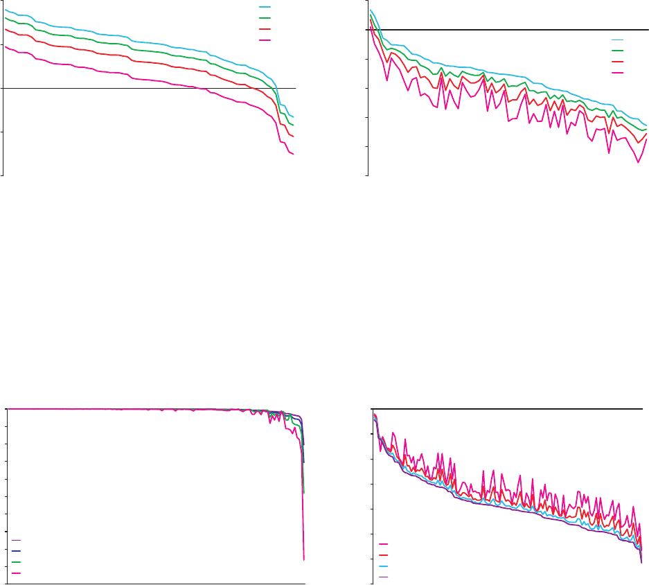
Figure 10.3 Loss of dryland (fraction of total area in 2000; panel(a)) and its value (percentage of GDP; panel(b)) without protection. Countries

are ranked as to their values in 2100.

Human-Induced Climate Change : An Interdisciplinary Assessment, edited by Michael E. Schlesinger, et al., Cambridge University Press, 2007. ProQuest Ebook Central,

http://ebookcentral.proquest.com/lib/wesleyan/detail.action?docID=321450.

Created from wesleyan on 2018-04-02 12:02:47.

0.01

0.1

100

Percent of area

2100

2075

2050

2025

0.00001

0.0001

0.001

0.01

0.1

Percent of area

2100

2075

2050

2025

Figure 10.4 Loss of wetland (fraction of total area in 2000; panel(a)) and its value (percentage of GDP; panel(b)) without protection (left

panels). Countries are ranked as to their values in 2100.

0.0

0.1

0.2

0.3

0.4

0.5

0.6

0.7

0.8

0.9

1.0

Fraction of land protected

2100

2075

2050

2025

0.0000001

0.000001

0.00001

0.0001

0.001

0.01

0.1

Percent of GDP

2025

2050

2075

2100

Figure 10.5 Protection level (fraction of coast protected; left panel) and the costs of protection (percent of GDP; right panel). Countries

are ranked as to their protection level.

Human-Induced Climate Change : An Interdisciplinary Assessment, edited by Michael E. Schlesinger, et al., Cambridge University Press, 2007. ProQuest Ebook Central,

http://ebookcentral.proquest.com/lib/wesleyan/detail.action?docID=321450.

Created from wesleyan on 2018-04-02 12:02:47.

Global Agro Ecological Zones (GAEZ)

AEZ1: Tropical, Arid

AEZ2: Tropical, Dry semi arid

AEZ3: Tropical, Moist semi arid

AEZ4: Tropical, Sub humid

AEZ5: Tropical, Humid

AEZ6: Tropical, Humid >300 day LGP

AEZ1: Temperate, Arid

AEZ2: Temperate, Dry semi arid

AEZ3: Temperate, Moist semi arid

AEZ4: Temperate, Sub humid

AEZ5: Temperate, Humid

AEZ6: Temperate, Humid >300 day LGP

AEZ1: Boreal, Arid

AEZ2: Boreal, Dry semi arid

AEZ3: Boreal, Moist semi arid

AEZ4: Boreal, Sub humid

AEZ5: Boreal, Humid

AEZ6: Boreal, Humid >300 day LGP

Figure 21.2 The global distribution of global agro-ecological zones (AEZ) from this study, derived by overlaying a global data set of

length of growing periods (LGP) over a global map of climatic zones. LGPs in green shading are in tropical climatic zones, LGPs in yellow-

to-red shading lie in temperate zones, while LGPs in blue-to-purple lie in boreal zones. LGPs increase as we move from lighter to dark

shades.

Human-Induced Climate Change : An Interdisciplinary Assessment, edited by Michael E. Schlesinger, et al., Cambridge University Press, 2007. ProQuest Ebook Central,

http://ebookcentral.proquest.com/lib/wesleyan/detail.action?docID=321450.

Created from wesleyan on 2018-04-02 12:02:47.

Harvested Area (million ha)

India China U.S.A. Russian Brazil

Federation

rice

wheat

pulses

millet

sorghum

rice

wheat

maize

soy

rape

soy

maize

wheat

cotton

sorghum

wheat

barley

rye

sunflowerseed

potatos

soy

maize

sugarcane

pulses

rice

Figure 21.5 The top ﬁve nations of the world, in terms of total harvested area, the top ﬁve crops and their harvested areas within each nation,

and the AEZs they are grown in. Tropical AEZs are shown in green, temperate in yellow-to-red, and boreal in blue-to-purple.

Atmospheric Chemistry

Ocean Carbon

Cycle

Energy

System

Climate

Ocean

Temperature

Sea level

Terrestrial

Carbon

Cycle

Crops &

Forestry

Hydrology

Unmanaged

Ecosystem

& Animals

Coastal

System

Agriculture,

Livestock &

Forestry

Atmospheric Composition

Climate and Sea Level

Human Activities

Ecosystems

Other Human

Systems

Figure 31.1 A schematic diagram of the major components of a climate-oriented integrated assessment model.

Human-Induced Climate Change : An Interdisciplinary Assessment, edited by Michael E. Schlesinger, et al., Cambridge University Press, 2007. ProQuest Ebook Central,

http://ebookcentral.proquest.com/lib/wesleyan/detail.action?docID=321450.

Created from wesleyan on 2018-04-02 12:02:47.

Scenarios

Assumptions

Policy Environment

Model

Analysis

Consequences

Economy

Climate

Figure 31.2 A schematic diagram of the elements of an IA model-based policy process.

Human-Induced Climate Change : An Interdisciplinary Assessment, edited by Michael E. Schlesinger, et al., Cambridge University Press, 2007. ProQuest Ebook Central,

http://ebookcentral.proquest.com/lib/wesleyan/detail.action?docID=321450.

Created from wesleyan on 2018-04-02 12:02:47.

Human-Induced Climate Change : An Interdisciplinary Assessment, edited by Michael E. Schlesinger, et al., Cambridge University Press, 2007. ProQuest Ebook Central,

http://ebookcentral.proquest.com/lib/wesleyan/detail.action?docID=321450.

Created from wesleyan on 2018-04-02 12:02:47.