Bank of England Staff Working Paper No. 713

Code of Practice

CODE OF PRACTICE 2007 CODE OF PRACTICE 2007 CODE OF PRACTICE 2007 CODE OF PRACTICE 2007 CODE OF

PRACTICE 2007 CODE OF PRACTICE 2007 CODE OF PRACTICE 2007 CODE OF PRACTICE 2007 CODE OF PRACTICE 2007

CODE OF PRACTICE 2007 CODE OF PRACTICE 2007 CODE OF PRACTICE 2007 CODE OF PRACTICE 2007 CODE OF

PRACTICE 2007 CODE OF PRACTICE 2007 CODE OF PRACTICE 2007 CODE OF PRACTICE 2007 CODE OF PRACTICE 2007

CODE OF PRACTICE 2007 CODE OF PRACTICE 2007 CODE OF PRACTICE 2007 CODE OF PRACTICE 2007 CODE OF

PRACTICE 2007 CODE OF PRACTICE 2007 CODE OF PRACTICE 2007 CODE OF PRACTICE 2007 CODE OF PRACTICE 2007

CODE OF PRACTICE 2007 CODE OF PRACTICE 2007 CODE OF PRACTICE 2007 CODE OF PRACTICE 2007 CODE OF

PRACTICE 2007 CODE OF PRACTICE 2007 CODE OF PRACTICE 2007 CODE OF PRACTICE 2007 CODE OF PRACTICE 2007

CODE OF PRACTICE 2007 CODE OF PRACTICE 2007 CODE OF PRACTICE 2007 CODE OF PRACTICE 2007 CODE OF

PRACTICE 2007 CODE OF PRACTICE 2007 CODE OF PRACTICE 2007 CODE OF PRACTICE 2007 CODE OF PRACTICE 2007

CODE OF PRACTICE 2007 CODE OF PRACTICE 2007 CODE OF PRACTICE 2007 CODE OF PR

ACTICE 2007 CODE OF

PRACTICE 2007 CODE OF PRACTICE 2007 CODE OF PRACTICE 2007 CODE OF PRACTICE 2007 CODE OF PRACTICE 2007

CODE OF PRACTICE 2007 CODE OF PRACTICE 2007 CODE OF PRACTICE 2007 CODE OF PRACTICE 2007 CODE OF

PRACTICE 2007 CODE OF PRACTICE 2007 CODE OF PRACTICE 2007 CODE OF PRACTICE 2007 CODE OF PRACTICE 2007

CODE OF PRACTICE 2007 CODE OF PRACTICE 2007 CODE OF PRACTICE 2007 CODE OF PRACTICE 2007 CODE OF

PRACTICE 2007 CODE OF PRACTICE 2007 CODE OF PRACTICE 2007 CODE OF PRACTICE 2007 CODE OF PRACTICE 2007

CODE OF PRACTICE 2007 CODE OF PRACTICE 2007 CODE OF PRACTICE 2007 CODE OF PRACTICE 2007 CODE OF

PRACTICE 2007 CODE OF PRACTICE 2007 CODE OF PRACTICE 2007 CODE OF PRACTICE 2007 CODE OF PRACTICE 2007

CODE OF PRACTICE 2007 CODE OF PRACTICE 2007 CODE OF PRACTICE 2007 CODE OF PRACTICE 2007 CODE OF

PRACTICE 2007 CODE OF PRACTICE 2007 CODE OF PRACTICE 2007 CODE OF PRACTICE 2007 CODE OF PRACTICE 2007

CODE OF PRACTICE 2007 CODE OF PRACTICE 2007 CODE OF PRACTICE 2007 CODE OF PRACTICE 2007 CODE OF

PRACTICE 2007 CODE OF PRACTICE 2007 CODE OF PRACTICE 2007

CODE OF PRACTICE 2007 CODE OF PRACTICE 2007

CODE OF PRACTICE 2007 CODE OF PRACTICE 2007 CODE OF PRACTICE 2007 CODE OF PRACTICE 2007 CODE OF

PRACTICE 2007 CODE OF PRACTICE 2007 CODE OF PRACTICE 2007 CODE OF PRACTICE 2007 CODE OF PRACTICE 2007

CODE OF PRACTICE 2007 CODE OF PRACTICE 2007 CODE OF PRACTICE 2007 CODE OF PRACTICE 2007 CODE OF

PRACTICE 2007 CODE OF PRACTICE 2007 CODE OF PRACTICE 2007 CODE OF PRACTICE 2007 CODE OF PRACTICE 2007

CODE OF PRACTICE 2007 CODE OF PRACTICE 2007 CODE OF PRACTICE 2007 CODE OF PRACTICE 2007 CODE OF

PRACTICE 2007 CODE OF PRACTICE 2007 CODE OF PRACTICE 2007 CODE OF PRACTICE 2007 CODE OF PRACTICE 2007

CODE OF PRACTICE 2007 CODE OF PRACTICE 2007 CODE OF PRACTICE 2007 CODE OF PRACTICE 2007 CODE OF

PRACTICE 2007 CODE OF PRACTICE 2007 CODE OF PRACTICE 2007 CODE OF PRACTICE 2007 CODE OF PRACTICE 2007

CODE OF PRACTICE 2007 CODE OF PRACTICE 2007 CODE OF PRACTICE 2007 CODE OF PRACTICE 2007 CODE OF

PRACTICE 2007 CODE OF PRACTICE 2007 CODE OF PRACTICE 2007 CODE OF PRACTICE 2007 CODE OF PRACTICE 2007

CODE OF PRACTICE 2007 CODE OF PRACTICE 2007 CODE OF PRACTICE 2007 CODE OF PRACTICE 2007 CODE OF

PRACTICE 2007 CODE OF PRACTICE 2007 CODE OF PRACTICE 2007 CODE OF PRACTICE 2007 CODE OF PRACTICE 2007

CODE OF PRACTICE 2007 CODE OF PRACTICE 2007 CODE OF PRACTICE 2007 CODE OF PRACTICE 2007 CODE OF

PRACTICE 2007 CODE OF PRACTICE 2007 CODE OF PRACTICE 2007 CODE OF PRACTICE 2007 CODE OF PRACTICE 2007

CODE OF PRACTICE 2007 CODE OF PRACTICE 2007 CODE OF PRACTICE 2007 CODE OF PRACTICE 2007 CODE OF

PRACTICE 2007 CODE OF PRACTICE 2007 CODE OF PRACTICE 2007 CODE OF PRACTICE 2007 CODE OF PRACTICE 2007

CODE OF PRACTICE 2007 CODE OF PRACTICE 2007 CODE OF PRACTICE 2007 CODE OF PRACTICE 2007 CODE OF

PRACTICE 2007 CODE OF PRACTICE 2007 CODE OF PRACTICE 2007 CODE OF PRACTICE 2007 CODE OF PRACTICE 2007

CODE OF PRACTICE 2007 CODE OF PRACTICE 2007 CODE OF PRACTICE 2007 CODE OF PRACTICE 2007 CODE OF

PRACTICE 2007 CODE OF PRACTICE 2007 CODE OF PRACTICE 2007 CODE OF PRACTICE 2007 CODE OF PRACTICE 2007

CODE OF PRACTICE 2007 CODE OF PRACTICE 2007 CODE OF PRACTICE 2007 CODE OF PRACTICE 2007 CODE OF

PRACTICE 2007 CODE OF

PRACTICE 2007 CODE OF PRACTICE 2007 CODE OF PRACTICE 2007 CODE OF PRACTICE 2007

CODE OF PRACTICE 2007 CODE OF PRACTICE 2007 CODE OF PRACTICE 2007 CODE OF PRACTICE 2007 CODE OF

PRACTICE 2007 CODE OF PRACTICE 2007 CODE OF PRACTICE 2007 CODE OF PRACTICE 2007 CODE OF PRACTICE 2007

CODE OF PRACTICE 2007 CODE OF PRACTICE 2007 CODE OF PRACTICE 2007 CODE OF PRACTICE 2007 CODE OF

PRACTICE 2007 CODE OF PRACTICE 2007 CODE OF PRACTICE 2007 CODE OF PRACTICE 2007 CODE OF PRACTICE 2007

CODE OF PRACTICE 2007 CODE OF PRACTICE 2007 CODE OF PRACTICE 2007 CODE OF PRACTICE 2007 CODE OF

PRACTICE 2007 CODE OF PRACTICE 2007 CODE OF PRACTICE 2007 CODE OF PRACTICE 2007 CODE OF PRACTICE 2007

CODE OF PRACTICE 2007 CODE OF PRACTICE 2007 CODE OF PRACTICE 2007 CODE OF PRACTICE 2007 CODE OF

PRACTICE 2007 CODE OF PRACTICE 2007 CODE OF PRACTICE 2007 CODE OF PRACTICE 2007 CODE OF PRACTICE 2007

CODE OF PRACTICE 2007 CODE OF PRACTICE 2007 CODE OF PRACTICE 2007 CODE OF PRACTICE 2007 CODE OF

PRACTICE 2007 CODE OF PRACTICE 2007 CODE OF PRACTICE 2007 CODE OF PRACTICE 2007 CODE OF PRACTICE 2007

CODE OF PRACTICE 2007 CODE OF PRACTICE 2007 CODE OF PRACTICE 2007 CODE OF PRACTICE 2007 CODE OF

PRACTICE 2007 CODE OF PRACTICE 2007 CODE OF PRACTICE 2007 CODE OF PRACTICE 2007 CODE OF PRACTICE 2007

CODE OF PRACTICE 2007 CODE OF PRACTICE 2007 CODE OF PRACTICE 2007 CODE OF PRACTICE 2007 CODE OF

PRACTICE 2007 CODE OF PRACTICE 2007 CODE OF PRACTICE 2007 CODE OF PRACTICE 2007 CODE OF PRACTICE 2007

CODE OF PRACTICE 2007 CODE OF PRACTICE 2007 CODE OF PRACTICE 2007 CODE OF PRACTICE 2007 CODE OF

PRACTICE 2007 CODE OF PRACTICE 2007 CODE OF PRACTICE 2007 CODE OF PRACTICE 2007 CODE OF PRACTICE 2007

Staff Working Paper No. 713

Down payment and mortgage rates:

evidence from equity loans

Matteo Benetton, Philippe Bracke and Nicola Garbarino

February 2018

Staff Working Papers describe research in progress by the author(s) and are published to elicit comments and to further debate.

Any views expressed are solely those of the author(s) and so cannot be taken to represent those of the Bank of England or to state

Bank of England policy. This paper should therefore not be reported as representing the views of the Bank of England or members of

the Monetary Policy Committee, Financial Policy Committee or Prudential Regulation Committee.

Staff Working Paper No. 713

Down payment and mortgage rates: evidence from

equity loans

Matteo Benetton,

(1)

Philippe Bracke

(2)

and Nicola Garbarino

(3)

Abstract

We present new evidence that lenders use down payment size to price unobservable borrower risk. We

exploit the contractual features of a UK scheme that helps home buyers top up their down payments with

equity loans. We ﬁnd that a 20 percentage point smaller down payment is associated with a 22 basis point

higher interest rate at origination, and a higher ex-post default rate. Lenders see down payment as a signal

for unobservable risk, but the relative importance of this signal is limited, as it accounts for only 10% of

the difference in mortgage rates between loans with 75% and 95% loan to value ratio.

Key words: Mortgage design, asymmetric information, leverage, housing policy.

JEL classiﬁcation: G21, R20, R30.

(1) London School of Economics. Email: [email protected]

(2) Bank of England. Email: philippe.brack[email protected]

(3) Bank of England. Email: nicola.garbarino@bankofengland.co.uk

We thank Saleem Bahaj, Joao Cocco, Scott Dennison, Paul Grout, John Mondragon, Antoinette Schoar, Marcus Spray and

Nikodem Szumilo, as well as seminar participants at the Bank of England for helpful comments and discussions. We also thank

the Department of Communities and Local Government, and the Homes and Communities Agency for providing data on

Help To Buy equity loans. Any views expressed are solely those of the authors and should not be taken to represent those of the

Bank of England or as a statement of Bank of England policy. This paper should not be reported as representing the views of

members of the Monetary Policy Committee or Financial Policy Committee.

The Bank’s working paper series can be found at www.bankofengland.co.uk/working-paper/Working-papers

Publications and Design Team, Bank of England, Threadneedle Street, London, EC2R 8AH

Telephone +44 (0)20 7601 4030 email publications@bankofengland.co.uk

© Bank of England 2018

ISSN 1749-9135 (on-line)

1 Introduction

Down payments are a ubiquitous feature of mortgage contracts (Stein, 1995). Interest

rates are higher on lower down payment mortgages to reﬂect higher risk (Bester, 1985; Adams

et al., 2009).

1

Low down payments can increase risk through two channels. First, low down

payments attract riskier borrowers (Campbell and Cocco, 2003, 2015; Corbae and Quintin,

2015). Second, a lower down payment also means less protection for the lender against falls

in the value of the housing collateral and a higher expected loss in case of borrower default

(Admati and Hellwig, 2014). Disentangling these two channels is fundamental to understand

whether lenders are concerned about the quality of the pool of borrowers or about house

price risk—both important channels that contributed to the ﬁnancial crisis (Mian and Suﬁ,

2009).

In this paper we study the causal eﬀect of down payment on interest rate through asym-

metric information. In other words, we isolate how lenders price the risk signal from down

payment size. We exploit the institutional features of a UK aﬀordable housing scheme that

oﬀers households equity loans to top up their down payment. The equity loans generate vari-

ation in down payment for mortgages with the same collateral, and hence the same expected

loss given default (LGD). In standard mortgages, a 20 percentage points lower down pay-

ment (from 75% to 95% loan-to-value ratio, LTV) increases the interest rate at origination

by about 200 basis points, but this combines the eﬀect of a higher default probability and

a higher LGD. Using our experiment, we ﬁnd that only 22 basis points can be attibuted to

unobservable borrower quality signalled by the down payment. We provide supporting evi-

dence that, ex-post, borrowers with 5% down payment are twice as likely to miss mortgage

payments than those with 25% down payment.

For the mortgage products that we study, our results suggest that lenders see down

payment as a signal for unobservable risk, but its relative importance is limited, as it accounts

1

Across countries, house buyers with a larger down payment get better mortgage rates (Al-Bahrani and

Su, 2015; Andersen et al., 2015; Benetton et al., 2017; Basten and Koch, 2015).

2

for only 10% of the diﬀerence in mortgage rates between loans with 75% and 95% LTV. This

is important for the innovative mortgage products that we study. Equity loans can make

house purchases more aﬀordable, in particular for households with limited down payment,

and may dampen the adverse macroeconomic eﬀects of house price volatility (Mian and

Suﬁ, 2015; Greenwald et al., 2017). The beneﬁts of equity loans would however be muted

if lenders charged substantially higher mortgage rates when households contribute only a

small portion of the equity.

We design an identiﬁcation strategy that exploits variation in down payment for the same

LGD, leveraging on the contractual features of the UK Help to Buy (HTB) Equity Loans

(EL) scheme. The scheme was introduced in 2013 and oﬀers households a 20% equity loan—

a contribution to the down payment to purchase a property—in exchange for a 20% share

of any future capital gains resulting from a sale of the property. The borrower contributes a

5% down payment. The mechanics of the contract is better explained with an example, that

we graphically show in Figure 1. Consider two mortgages with a 75% loan-to-value ratio: a

“standard” mortgage where the borrower pays a 25% deposit; and a EL where the borrower

pays only a 5% deposit and the remaining 20% is provided by the scheme. The loan-to-value

on the two mortgages is the same, and, from the bank’s perspective, there is no diﬀerence in

terms of LGD. But the down payment from the borrower is diﬀerent, and we test whether

this diﬀerence aﬀects pricing.

Our novel dataset contains about 92,000 mortgages originated between April 2013 and

June 2016 and combines information on the EL scheme (from the Homes and Communities

Agency), mortgage origination and performance (Financial Conduct Authority) and house

prices (Land Registry).

We create two groups of borrowers with diﬀerent down payments but same LGD and

we test whether the group with the lower down payment pays a higher mortgage rate,

controlling for observable borrower and product characteristics. These characteristics capture

the hard information used in mortgage pricing and available to both the lender and the

3

econometrician. Soft information (observable to the lender, but not to the econometrician)

is unlikely to matter given the centralized pricing strategies in the mortgage market—the

UK mortgage market is a “supermarket”, with standardised products priced on a limited

number of variables (Benetton, 2017).

We ﬁnd a 16 basis points premium on EL mortgages when we compare the interest rates

on EL mortgages and “standard” 75% loan-to-value mortgages. As expected, we ﬁnd a large

diﬀerence in terms of the size of the down payment (in monetary terms), while diﬀerences

in terms of house prices and borrower characteristics, such as age and income, are more

muted. Compared to standard borrowers, EL borrowers purchase, on average, houses that

are £21,000 (8%) cheaper but their down payment is £51,000 (80%) smaller. The EL

premium increases to 22 basis points when we compare EL and standard mortgages issued

by the same lender, in the same period, with the same product characteristics (eg. ﬁxed vs

variable mortgage rate). These are the main characteristics on which mortgages are priced

in the UK market. The premium is robust to additional regional and borrower controls that

are not explicitly priced but could vary between EL and standard mortgages. Only when we

control for the down payment the EL premium disappears.

To corroborate our story based on higher unobservable risk we test whether EL borrowers

with a low down payment also have a higher delinquency rate than borrowers with standard

mortgages and similar loan-to-value ratios. We ﬁnd that delinquency rates are higher for EL

mortgages compared to standard 75% loan-to-value mortgages. Finally, we assess competing

explanations for the diﬀerence in mortgage rates between the two groups. We test whether

there is less bank competition in the supply of EL mortgages or whether properties bought

with EL have a higher depreciation risk, but these explanations are not supported by the

data.

Related literature. Our paper contributes to two related streams of literature. First,

we contribute the household ﬁnance literature that looks at mortgage products (see among

others Campbell and Cocco, 2003; Guiso et al., 2013; Campbell and Cocco, 2015). The 2008

4

crisis has revamped the debate about optimal mortgage design (Cocco, 2013; Campbell, 2013;

Miles, 2015), and several recent papers have suggested and analyzed alternative mortgage

products, such as shared appreciation mortgages (Shiller, 2007; Greenwald et al., 2017);

option adjustable rate mortgages (Piskorski and Tchistyi, 2010); ﬁxed rate mortgages with

underwater reﬁnancing (Campbell, 2013); and convertible ﬁxed rate mortgages (Eberly and

Krishnamurthy, 2014). We build on this literature and study a new government scheme

designed to promote aﬀordability in the UK mortgage market by providing an equity loan

to the borrower. We look at the supply side and study how lenders react to the scheme by

adjusting their pricing strategy.

Second, our work contributes to the literature that tests empirically whether lenders

use collateral as a screening device (Adams et al., 2009). Despite the importance of the

mortgage market, this paper is, to our knowledge, the ﬁrst to look at how down payment is

used as a screening mechanism in this context. Most of the literature uses collateral data

to evaluate corporate or small-medium enterprise lending—see Berger et al. (2011) for a

survey. For households, Adams et al. (2009) analyse the relationship between down payment

and borrower quality in the market for subprime car loans; while Agarwal et al. (2016)

study home equity loans and ﬁnd that less creditworthy borrowers choose contracts with less

collateral. Our identiﬁcation approach exploits contractual features of mortgages to estimate

the eﬀect of information asymmetries on pricing, along the lines of recent papers by Ambrose

et al. (2016) and Hansman (2017). Similarly to these paper we look at the eﬀect of down

payment on contract choice and default, but we also consider how this is reﬂected on pricing

and disentangle the probability of default from LGD with an innovative research design.

The rest of the paper is organized as follows. Section 2 describes the setting and the

data. Section 3 presents our indentiﬁcation strategy and shows the main result. In Section

4 we discuss additional evidence on mortgage performances and alternative explanations for

our ﬁndings. Section 5 concludes.

5

2 Setting and data

EL is a UK shared equity scheme that allows households to buy new properties with a

lower down payment. In this section we highlight the importance of down payment in the

UK mortgage market and explain how the EL scheme works. We also show that, in the

data, a lower down payment is associated with higher mortgage rates and more frequent

delinquencies.

2.1 The UK mortgage market

In international context, the UK mortgage and housing markets are characterised by high

household indebtedness, medium levels of home ownership, and adjustable rate contracts

with short initial ﬁxed-rate periods (Campbell, 2013; Jord`a et al., 2016).

Mortgage originations Since April 2005 UK mortgage lenders have been required to

report all their mortgage originations to the Financial Conduct Authority (the Financial

Services Authority until 2013). The submissions include detailed information on loan, bor-

rower and property characteristics. This information is collected in the FCA’s Product Sales

Data (PSD), on which we base our analysis.

2

In the UK mortgage leverage—as measured by the LTV ratio—is driven by the size of

the down payment rather than the value of the house. Figure 2 uses the full set of PSD

originations to show the distribution of house values and down payments by LTV. The

average house price is relatively ﬂat (about £200,000) up to 75% LTV and then decreases

gradually. The average down payment instead falls steadily with LTV.

Moreover, UK lenders set an interest rate schedule that increases with the LTV. Mort-

gages are priced on a limited number of variables, typically LTV, borrower type (ﬁrst-time

2

The PSD includes remortgages and excludes buy-to-let mortgages. Some of the variables contained in

the PSD are: borrower type (ﬁrst-time buyer, home mover, remortgagor), age, income, loan value, loan-

to-income ratio (LTI), maturity, product type (e.g. ﬁxed, ﬂoating), property value, location (full six-digit

postcode).

6

buyer, home mover, remortgager) and rate type (length of ﬁxed period). Other indicators of

borrower quality, such as loan-to-income and credit rating are used to approve or reject the

application, but do not aﬀect mortgage rates.

3

To demonstrate the importance of LTV for

UK mortgage rates, we follow Best et al. (2015) and regress the interest rate at originations

on a set of product and time dummies and LTV bins. Figure 3 shows the results. The

conditional interest rate increases with discrete jumps at the relevant LTV thresholds. The

jumps in the interest rate are largest for LTVs above 85 and 90.

Mortgage performance data Since summer 2015 UK mortgage lenders have been re-

quired by the FCA to provide a loan-level snapshot of their current mortgage holdings. These

mortgage performance data are part of the PSD and include a number of loan characteris-

tics, such as date of origination, original and current loan balance, remaining mortgage term,

and whether the mortgage has ever been delinquent.

4

We deﬁne delinquent borrowers (or

borrowers in arrears, in UK terminology) as those that missed payments for a total amount

exceeding the value of three regular monthly payments.

We use the mortgage performance data in Section 4 where we evaluate the repayment

performance of EL borrowers against other purchasers of equivalent, non-EL mortgages. We

employ the snapshot of owner-occupied mortgages as of December 31, 2016 and single out

loans that have been in arrears at least once since origination.

In general, mortgages with higher leverage (and hence lower down payment) are more

likely to be delinquent. Figure 4 shows that the proportion of delinquent borrowers increases

more than proportionally with LTV. This fact holds both unconditionally (Figure 4a) and

when we control for a rich set of borrower and loan characteristics (Figure 4b).

3

Moreover, rates are not dependent on the location of the property.

4

These variables do not perfectly overlap with the ones in the origination data, but the two datasets can

be combined by matching on the postcode and date of birth of the borrower.

7

2.2 Help To Buy - Equity Loan scheme

The UK government started the EL scheme in April 2013, with the objective of supporting

“creditworthy but liquidity constrained” households and increase the supply of new housing.

5

The government originally planned to phase out the scheme in 2016, but it has now extended

it until 2021. The scheme is available in England and Wales. A similar, but separate, scheme

is available in Scotland.

While there had been other schemes to support home ownership prior to EL, these were

on a smaller scale. For example, its immediate predecessor, FirstBuy, had a budget of £250

million. The UK government initially set a maximum budget for EL of £3.7 billion. In

October 2017 it pledged a further £10 billion and promised to continue to scheme until

2021.

The EL scheme provides an equity loan of up to 20% of the value of the house. In

exchange, the scheme receives interest and participates in any capital gains or losses resulting

from the sale of the property. To be eligible, the borrower has to provide a minimum 5%

down payment. The bank or building society provides a mortgage for the remaining balance

(up to 75%).

6

In case of default, the HTB-EL scheme holds a “second charge” on the

property. The proceeds from a sale of the property go ﬁrst to the bank or building society

that provided the mortgage.

Eligibility is not subject to income restrictions and there are no checks on whether the

borrower could provide a larger down payment. However, borrowers must meet aﬀordabil-

ity requirements to ensure that they will be able to repay the mortgage.

7

The scheme is

5

First-time buyers and new builds were particularly aﬀected by the housing downturn of 2007-08. The

supply of high LTV mortgage in the UK fell sharply following the crisis of 2007-08, as mortgage lenders

sought to reduce credit risk. First-time buyers experienced an increase in the average down payment (15%

pre-crisis to over 25% in 2010) and a fall in mortgage lending (which halved between 2007 and 2008). Younger

households were aﬀected most. In 1991, 67% of the 25 to 34 age group were homeowners. By 2014, this

had declined to 36% (Oﬃce for National Statistics, 2016). The sharp fall in house prices also aﬀected house

construction, which fell from over 200,000 per annum in 2007 to less than 150,000 in 2010 . Demand was

constrained by limited mortgage availability for new properties, in particular at high LTVs.

6

The description of the HTB-EL scheme is based on National Audit Oﬃce (2014), (Gov.uk, 2016a) and

(Gov.uk, 2016b).

7

These include, for instance, a 4.5 loan-to-income (LTI) limit based only on the mortgage. The aﬀordabil-

8

available to both ﬁrst-time buyers and home movers, but not for second homes or buy-to-let

investment. The property must have a purchase price of £600,000 or less. The borrower has

to pay to the scheme only a £1 fee for the ﬁrst ﬁve years. After that, the annual interest fee

is 1.75%, increasing each year with the Retail Price Index (RPI). Payments of this fee do not

amortize the equity loan capital. The borrower can make principal repayments at any time.

The minimum repayment is 10% and is calculated on the basis of the market valuation of

the house.

8

The borrower must repay the full value of the loan when the property is sold or

after a maximum of 25 years.

The scheme is administered by the Department for Communities and Local Government

(DCLG) and the Homes and Communities Agency (HCA) through a network of local agents,

who process the applications. EL operates under slightly diﬀerent criteria in Wales and the

Greater London area. In Wales, the maximum property price is £300,000.

9

In London, the

EL limit was increased from 20% to 40% in February 2016.

10

We exclude Wales and London

(after January 2016) from our analysis.

EL originations and performance data We obtained from the HCA the complete

database of all EL loans for the ﬁrst 39 months of the scheme, from April 2013 to June 2016.

The dataset includes 91,759 loans with information on full postcode, size of the mortgage,

purchase price, lender name, and expected completion date.

Appendix Table 7 shows descriptive statistics for the EL dataset. The total value of these

equity loans is £4.17 billion, whereas the total value of properties sold under the scheme is

£20.82 billion. According to the England and Wales Land Registry there were 286,593 sales

of new properties in England between April 2013 and June 2016, implying that one third of

ity measures do not include the equity loan. One possible reason for the low EL premium that we measure

on mortgage rates could be that lenders take reassurance from the additional checks that the Government

carries out on borrowers. However, given that there is no additional requirement on borrowers compared to

other mortgages, and the LTI constraints are in fact eased by the equity loan, this eﬀect is likely to be small

or nonexistent.

8

For example, if the value of the property has increased from £200,000 to £220,000 the minimum repay-

ment is £22,000.

9

See (Welsh Government, 2016).

10

See (HM Government, 2016).

9

the new build market was ﬁnanced by EL. Since new builds correspond to approximately 10

percent of all housing transactions, EL ﬁnanced 3 percent of all housing sales in England.

We match the EL dataset to the PSD to identify mortgage originations that are asso-

ciated with an EL.

11

We then restrict our analysis to two groups of borrowers with the

same collateral but diﬀerent down payment. The ﬁrst group is composed of EL borrowers

that contribute with a 5%-10% down payment (with the vast majority putting down the

minimum 5%—see Appendix Figure 8), while the scheme ﬁnances an additional 20% of the

purchase price. The second group is composed of borrowers that contributed a 25%-30%

down payment with a standard 70-75% LTV mortgage. For simplicity, from now on we refer

to the ﬁrst group as EL borrowers and second group as “standard” borrowers.

12

Table 1 shows descriptive statistics for EL and standard borrowers, while Figure 5 shows

the diﬀerent distributions of house purchase prices, incomes, mortgage sizes, and down pay-

ments. By construction, the size of the down payment constitutes the main diﬀerence be-

tween the EL and standard borrowers. EL allows borrowers to purchase similar (but slightly

cheaper) houses with similar (but slightly smaller) mortgages. Table 1 also shows that EL

borrowers are younger and have lower incomes, are more likely to be ﬁrst time buyers, and

are less likely to buy a property in London.

As an anticipation of the main result of this paper, we show in Table 1 that the aver-

age interest for the EL group is 11 basis points (4%) higher than for standard borrowers.

Moreover, EL borrowers are more likely to become delinquent: the delinquency rate for EL

borrrowers is 0.29%, almost double the rate for the standard borrowers (0.15%).

13

As with the universe of UK mortgages, in our subsample of interest we observe a cor-

relation between down payment, mortgage rates, and delinquencies. In this sample we can

exclude that the correlation between down payment and mortgage rates is caused by diﬀer-

ent losses in the event of default, which are set equal for all loans, suggesting that that the

11

Data cleaning and matching are described in Appendix Table 8.

12

These groups are neither the universe of EL borrowers (a few EL borrowers contribute a down payment

higher than 5%) nor that of “standard” mortgages (we exclude mortgages with other LTVs).

13

Given the recent introduction of the EL scheme (2013), the number of loans in arrears is limited. In our

sample, 110 EL borrowers are in arrears, compared to 24 standard borrowers.

10

EL premium is driven by the higher default risk of low down payment borrowers. In the

next section, we develop an identiﬁcation strategy to test whether the correlation between

down payment and mortgage rates is robust to controlling for observable borrower and loan

characteristics.

3 Down payment and mortgage rates

Theories of collateral as a screeening mechanism predict that lower collateral—in the

case of mortgages, down payment— should be associated both with higher interest rate and

higher risk (Bester, 1985). In this section we measure the eﬀect of collateral on mortgage

rates, while in section 4 we focus on mortgage delinquencies.

3.1 Hypothesis

The mortgage rate r needs to compensate for the risk the borrower will not repay in

full, which depends on the probability of non-repayment p and on the loss in case of non-

repayment l. The mortgage rates also need to compensate operational costs c and a mark-up

m:

14

r = p(X, d) · l(∆h, d) + c + m. (1)

The probability of non-repayment p is a function of observable X and non-observable χ

risk characteristics: p = p(X, χ). If the down payment d is a signal of non-observable risk

(d = d(χ)), then: p = p(X, d).

The down payment however aﬀects the interest rate in another way, too. In case of

default, the lender can repossess the property. The lender incurs a loss if the current value

the property is below the value of the outstanding loan, which can happen if the fall in house

value ∆h is larger than the orginal down payment d.

14

The components l, c and m are all expressed as a proportion of the loan. We do not assess whether

lenders are pricing risk correctly.

11

Equation (1) highlights our channel of interest and the main confounding factors that

we need to control for. All else equal, we expect lower d to be associated with (a) higher

mortgage rates r and (b) higher risk p.

3.2 Research design

Our goal is to establish a causal link from down payment to interest rate, only through

default risk. This objective requires us to observe the interest rates for two identical mort-

gages by the same lender, for the same property, taken by two borrowers who diﬀer only

in the size of the down payment. This is unlikely in most mortgage markets because, even

conditioning on all observable borrower and mortgage characteristics, a lower down payment

aﬀects interest rates through both p and l in equation (1).

To isolate empirically the eﬀect of d through unobservable risk χ we proceed as follows.

First, we keep l constant by comparing the two groups of mortgages, EL and standard (as

deﬁned in the previous section), with the same collateral but diﬀerent down payment and

adding regional ﬁxed eﬀects to control for house price volatility ∆h. Second, to remove

variation in operational costs c and mark-up m we add interacted product-time ﬁxed eﬀects,

which also remove diﬀerences in risk across products and time. Third, we control for observ-

able risk X by adding exogenous borrower characteristics. At this point, we attribute any

remaining EL premium after introducing these controls to the lower down payment provided

by EL borrowers. As a last step, we check this by introducing the down payment d in the

regression and verifying that the EL premium disappears.

We estimate the following model:

r

ijkt

= αEL

i

+ β

jt

+ γ

k

+ δX

i

+ ηZ

i

+ 

ijt

(2)

where r

ijkt

is the interest rate paid at origination by borrower i for product j in month t to

purchase a property in region k; EL

i

is a dummy variable equal to one if the mortgage is under

12

the government scheme; β

jt

are interacted product-time ﬁxed eﬀects;

15

γ

k

are geographic

ﬁxed eﬀects. X

i

are exogenous borrower characteristics and Z

i

are additional borrower

controls—house prices and down payment.

Our coeﬃcient of interest is α which captures the EL interest rate premium. Our hy-

pothesis is that that α falls to zero only when we add the down payment as a control, but

remains positive otherwise.

3.3 Results

Table 2 presents our main result on mortgage rates. We test diﬀerent explanations for

the interest rate diﬀerential shown in section 3.2 by gradually introducing the controls in

equation (2).

Column (1) in Table 2 shows the regression of the loan-level interest rate on the EL

dummy. As shown in the descriptive stats in Section 2.2, lenders on average set an interest

rate that is 11 basis points higher for HTB-mortgages than for mortgages within the same

LTV band.

In column (2) we add the interacted product-time ﬁxed eﬀects (β

jt

) to control nonpara-

metrically for diﬀerences in product characteristics. We exploit only the variation in interest

rate within product-month-LTV, eﬀectively comparing the interest rate on mortgages oﬀered

by the same lender, in the same month, to the same borrower type (ﬁrst-time buyer vs. home

mover) at the same conditions (e.g. ﬁxed rate for two years). We ﬁnd that the EL premium

increases to 22 basis points.

In column (3) we include geographic ﬁxed eﬀects γ

k

. The EL premium may be driven

by local factors if borrowers with EL mortgages tend to buy houses in locations with higher

house price volatility or macroeconomic risk. However, when adding geographic ﬁxed eﬀects,

we ﬁnd that the coeﬃcient on the EL dummy decreases by only 1 basis point.

In column (4) we control for exogenous borrower characteristics (X

i

). We include age and

15

A product in our setting is the combination of a lender, an interest rate type (e.g. ﬁxed or variable) and

a borrower type (ﬁrst time buyer, home mover).

13

income of the borrower, employment status (employee or self-employed) and type of mortgage

application (joint- or single-income application). Even if mortgage pricing in the UK is not

borrower speciﬁc, selection into certain types of products can aﬀect the pricing strategy of

lenders (see section 2). If low-income borrowers systematically choose EL mortgages, the

higher interest rate associated to EL will capture the eﬀect of lower income. The EL premium

stays stable at about 22 basis points.

In our data we are unable to observe all the information that lenders have on borrower

risk characteristics. For example, we do not have data on credit scores. As explained in

Section 2.1, this additional information is not used directly to price UK mortgages, but

may aﬀect pricing indirectly through average borrower risk. However, we note that adding

observable borrower characteristics to the regression has a small eﬀect on the EL premium,

suggesting that product ﬁxed eﬀects are able to absorb a substantial amount of variation in

borrower risk characteristics.

Finally, we control for additional borrower variables (Z

i

) to test our main mechanism. In

column (5) we add the house value to compare mortgages for houses with similar prices, in

the spirit of Figure 1. The EL premium remains around 22 basis points. Income becomes

insigniﬁcant when we add house value, due to the high correlation between the two variables.

In column (6) we control for loan size instead of house price. Given that we restrict the

estimation sample to loans with the same LTV, controlling for house value or loan size yields

the same result.

In column (7) we add down payment to the regression in order to test explicitly whether

diﬀerences in down payment explain the interest rate diﬀerence between EL and standard

borrowers with similar LTV, mortgage product, and houses. The price diﬀerence between

EL and standard borrowers decreases by 10 basis points. Finally in column (8) we allow the

down payment to enter nonlinearly in the model, making the whole EL premium insigniﬁcant.

To summarise, the size of the down payment provides information on borrowers over and

above their risk characteristics and housing choices. We ﬁnd that lenders price EL mortgages

about 22 basis point higher than equivalent standard mortgages. This premium is explained

14

by the lower down payment. In our restricted sample, the down payment contributed by EL

borrowers is 20 percentage points lower than that contributed by standard borrowers (5%

and 25% respectively)—a diﬀerence of about £50,000.

Heterogeneity Table 3 shows the results on heterogeneity in EL mortgage rates across

borrowers and lenders. In the ﬁrst two columns of the table we compare ﬁrst-time buyers

and home movers. The EL premium is larger for home movers by about 10 basis points.

This ﬁnding may seem counterintuitive given that ﬁrst-time buyers have no credit history in

the mortgage market. However, the inability to make a large down payment seems to carry

a particularly bad signal for home movers, who may have had the possibility to build equity

with their previous house.

In the remaing columns of Table 3, we study heterogeneity across lenders. Previous

studies have shown that pricing of risk can vary with lender characteristics, such as size and

funding structure (He et al., 2012; Jim´enez et al., 2014; Dagher and Kazimov, 2015). In

columns (3) and (4) of Table 3, we look at lender size. We compare the top four lenders in

our sample with the smaller lenders and building societies. The EL premium for the lenders

accounting for the vast majority of originations is close to the baseline of 20 basis points,

as expected. The other lenders charge EL mortages more, at almost 35 basis points. This

diﬀerence can be attributed to both demand and supply factors. Borrowers taking EL from

smaller lenders may be relatively riskier than the standard borrowers. Alternatively, smaller

lenders may be more cautious in pricing unobservable risk.

For the largest lenders we collect additional information on their capital buﬀers and fund-

ing costs. In columns (5) and (6) of Table 3 we study heterogeneity based on capital buﬀers,

deﬁned as the diﬀerence between a bank’s capital resources and the minimum regulatory

capital requirement (both measured as a percentage of total assets). We ﬁnd that the EL

premium is almost 30 basis points for lender with a low buﬀer and around 12 basis points

for lenders with a larger buﬀer. Better capitalized lenders pass on the scheme to borrowers

at lower prices. Moreover, this result seems to suggest that lenders with lower capital do not

15

extend cheap credit to riskier borrowers, in contrast with recent evidence in other settings

(Jim´enez et al., 2014).

Columns (7) and (8) of Table 3 compare lenders with diﬀerent funding costs, which we

proxy with data on lenders’ credit default swaps. We ﬁnd that for lenders with high funding

costs the EL premium reaches 34 basis points, while lenders with low funding costs price it

at about 16 basis points. Lenders with lower funding costs pass on the scheme to borrowers

at lower prices.

4 Down payment and risk

In the previous section we showed that lenders price EL mortgages higher than equivalent

standard mortgages and the diﬀerence is due to unobservable factors related to the size of the

down payment. In this section, we provide evidence that EL mortgages are ex-post riskier,

consistent with our main ﬁnding of an EL premium in mortgage rates. We also address

alternative mechanisms that could explain the premium.

4.1 Ex-post performance

In equation (1), the down payment aﬀects the mortgage rate because it signals unob-

servable borrower characteristics that increase the probability of default. But to extract

the signal, the lender must observe that, all else equal, lower down payment borrowers are

ex-post riskier. In Section 2.2 we have shown that, unconditionally, EL borrowers are twice

as likely to become delinquent than standard borrowers. In this section we show that this

relation holds after controlling for observable borrower and loan characteristics.

To measure the eﬀect of down payment on ex-post performance controlling for confound-

ing factors, we estimate a model similar to (1) but with the probability of delinquency as

dependent variable. This takes the form of the following probit model:

Delinquent

ilt

= βEL

i

+ γ

l

+ γ

t

+ αZ

i

+ δX

i

+ 

ilt

. (3)

16

where Delinquent

ilt

is a dummy equal to one if borrower i has been delinquent at any point

before the end of 2016. Our coeﬃcient of interest is β which captures the additional risk

associated with EL mortgages; with this variable we aim to isolate only the eﬀect of the

unobservable risk on delinquencies that the borrower signals via a lower down payment. To

control for other factors aﬀecting the probability of delinquency we include a full set of year

of origination and lender ﬁxed eﬀects, borrower and property level controls. We also estimate

(3) with the interest rate at originations (r

ijt

) among the controls, although the results of

this specﬁication have to be taken with caution, given the endogenous nature of mortgage

rates.

Table 4 presents the results. Column 1 replicates the unconditional marginal eﬀect of EL

on the delinquency rate (0.13 percentage points). In column 2-4 we add similar controls to

those in the price regression in Table 2. We incrementally add year and region ﬁxed eﬀects

(column 2), borrower characteristics and house value (column 3) and lender ﬁxed eﬀects

(column 4). Due to the limited number of observed delinquencies, we use separate lender

and year ﬁxed eﬀects rather than the full set of product-by-month ﬁxed eﬀects. We ﬁnd that

the eﬀect of EL on the delinquency rate remains around 0.10 percentage points, and is still

signiﬁcant at the 10% level, despite the small number of delinquencies in the sample.

In the last column of Table 4 we show the results including the mortgage interest rate

in the regression. This speciﬁcation checks that the diﬀerent delinquency probabilities be-

tween EL and standard borrowers are not simply due to the fact that EL borrowers pay

higher rates (as shown in the previous section) and therefore have a harder time servicing

their mortgage. However, mortgage rates are themselves an endogenous outcome variable,

which hinders the interpretation of the conditional eﬀects estimated by the regression: EL

borrowers are charged more precisely because of their higher delinquency probability. With

this caveat in mind, column 5 shows that EL borrowers are still 0.07 percentage points more

likely to become delinquent than standard borrowers, but the diﬀerence is now statistically

insigniﬁcant.

What unobservable risk characteristics does the down payment signal? Our ﬁnding of a

17

higher delinquency rate for EL borrowers could be due to either lower borrower quality at

origination or stronger incentives to default due to higher leverage. Under the ﬁrst interpre-

tation, borrowers that are illiquid today are also likely to be illiquid tomorrow, and unable

to pay in case of income shock (Adams et al., 2009). This intuition can be formalised in

models where households save for precautionary reasons. In Campbell and Cocco (2003) and

Campbell and Cocco (2015) impatient mortgage borrowers with a higher discount rate accu-

mulate a smaller buﬀer stock on liquid ﬁnancial assets and are more likely to miss mortgage

payments.

Under the second interpretation, EL borrowers are more leveraged and hence more likely

to fall into negative equity than the control group. For example, a fall in property value from

£100,000 to £90,000 would be suﬃcient to push into negative equity a HTB borrower with

a £5,000 deposit at origination, but not a standard 75-percent LTV mortage with £25,000

equity at origination. This higher leverage increases the probability of negative equity and

hence the opportunities for strategic default (for a recent example see Hansman (2017)).

It is worth pointing out, however, that the incentive to strategically default are not as

high for EL borrowers as for other homeowners that put a 5% down payment. Figure 6

shows how the equity position of borrowers varies depending on house prices and type of

mortgages, assuming an initial house value of 100. For simplicity, we assume an interest

only mortgage, where payments cover only the interest and none of the principal is repaid

until sale. The initial equity of EL owners is the same as that of 95%-LTV borrowers, but

its sensitivity to house price movements is lower. Because of the cushion provided by the

government scheme, the EL household will reap lower gains for any increase in house value,

but will also suﬀer lower losses for any house price decline. It takes a fall in house prices of

more than 6.25% for a EL borrower to be in negative equity.

16

Two additional considerations point towards a bigger role for borrower quality as opposed

to strategic defaults. First, between 2013 and 2016 average house prices grew across all

16

In the simpliﬁed case of an interest-only mortgage, EL borrower equity is E

t

= 0.8HP

t

− Q

t

= 0.8HP

t

−

0.75HP

0

, where HP

t

and Q

t

are, respectively, the house price and the outstanding mortgage balance at the

end of the period, while HP

0

is the purchase price of the house.

18

regions in England. All 370 local authorities experienced an increase in house prices except

for Redcar and Cleveland (in North East England) and Allerdale (in North West England).

17

Therefore arrears in our sample are not driven by strategic defaults.

Second, the UK framework for treating mortgages in default is full recourse. UK mort-

gage borrowers can be pursued for up to six years for any remaining mortgage obligation

(Lambrecht et al., 2003; Aron and Muellbauer, 2016). They remain liable for their debt even

after the property has been reposessed by the lender, if the sale value of the property does

not cover the value of the debt. Lambrecht et al. (2003) ﬁnd that UK lenders’ foreclosure

decisions depend more on cash ﬂow shocks (income, interest rates) than on leverage.

18

Evi-

dence for the US indicates that full recourse signiﬁcantly reduces, but does not completely

eliminate, incentives for strategic default (Ghent and Kudlyak, 2011).

We conclude with a back-of-the-envelope calculation of the eﬀect of down payment on

mortgage rates. Borrowers for EL mortgages put the same down payment (5%) as borrower

of 95%-LTV mortgages. However, 95%-LTV mortgages entail a signiﬁcantly diﬀerent LGD

for lenders. Figure 3 shows that in the UK the average diﬀerence in mortgage rates between

75 and 95%-LTV mortgages is around 200 basis points. In this paper we show that borrowers

who put only a 5% down payment pay, ceteris paribus, a mortgage rate premium of 20 basis

points. We can therefore conclude that probability of default explains approximately 10% of

the diﬀerential between 75 and 95%-LTV mortgages, with the bulk of the diﬀerential (90%)

explained by diﬀerences in LGD.

4.2 Alternative explanations

The analysis in section 4.1 is consistent with an interpretation of the EL premium in

terms of default risk, driven by ex-ante selection. But our results could also be consistent

with alternative mechanisms. First, the EL premium could also reﬂect higher repayment

17

We checked local house price trends using the house price indices available at https://www.gov.uk/

government/statistical-data-sets/uk-house-price-index-data-downloads-march-2017.

18

This is conﬁrmed by regulatory surveys in which strategic default does not seem to be a concern for

lenders operating in the UK market.

19

risk. Second, the premium could be compensating lenders for higher depreciation risk for

EL properties. Third, the EL premium could reﬂect a markup due to lower competition in

the EL segment, compared to standard mortgages, within the new build market. We explore

each explanation in turn, but ﬁnd limited evidence in their support.

Lenders are exposed to the risk that the borrower terminates the contract early to reﬁ-

nance at a lower rate (Campbell and Cocco, 2003). The borrowers in our sample have an

incentive to reﬁnance at the end of the ﬁxed-rate period (typically two or ﬁve years) after

which the mortgage rate reverts to a higher “standard variable rate” (Miles, 2004). The

original lender receives lower cash ﬂows, compared to the standard variable rate, if it oﬀers

a new ﬁxed-rate contract, but loses all future cash ﬂows if the borrower switches to another

provider or sells the property. The descriptive statistics in Table 1 however indicate that,

unconditionally, EL borrowers are less likely than standard borrowers to reﬁnance or sell the

house.

19

. We test this result by substituting reﬁnancing and sale as the dependent variables

in probit regressions similar to Equation 3. The results in Table 5 indicate that diﬀerences

between the two groups in the probability of resale or reﬁnance with the same bank are

either not signiﬁcant. The diﬀerence is statistically signiﬁcant but economically marginal in

the case of reﬁnance with another bank (EL borrowers are slightly less risky).

New houses usually sell at a premium compared to other properties of comparable char-

acteristics.

20

For our identiﬁcation strategy, this premium is only problematic to the extent

that it aﬀects EL properties more than other equivalent new builds. This diﬀerential impact

could be due to: (1) lower price elasticity of EL buyers, (2) less maintenance eﬀort by EL

buyers (possibly because of the risk sharing component of the EL contract as in Shiller and

Weiss, 2000), or (3) developers using EL as an alternative to the variety of incentives that

have been on oﬀer to other buyers, which might include discounts to list price, or higher

speciﬁcations of homes or features.

21

19

We consider all reﬁnancing ans sales activity between origination and the end of 2016.

20

“[H]ouses are a bit like new cars, which lose value immediately upon being driven oﬀ the lot.” (Coulson

et al., 2016)

21

EL mortgages could be issued in areas with higher house price volatility, and this would also induce

higher depreciation. However, our geographic ﬁxed eﬀects address this problem.

20

To check that our results are not driven by depreciation risk, we identify which proper-

ties in the treatment and control group were resold within the sample period. We match

the PSD mortgage ﬂow dataset with the England and Wales Land Registry and ﬁnd 485

cases of sales (186 in the control group and 299 in the treatment group). We compute the

appreciation of properties as the (log) ratio between the transaction price at sale and the

purchase price. Table 6 shows that, unconditionally, EL properties have lower appreciation

rates, by approximately four percentage points. However, once we control for purchase year,

or for purchase year and sale year, the diﬀerence becomes insigniﬁcant. Additional controls

for region ﬁxed eﬀects drive the diﬀerence close to zero.

Lower competition in the EL market compared to standard mortgages on new builds

could lead to a higher markup for EL mortgages. For example, the administrative burden

associated with oﬀering EL mortgages could inhibit entry by some lenders, especially smaller

banks. Mortgages lenders interviewed as part of DCLG (2016)’s evaluation of the EL scheme

indicate that mortgage lending for the new build market is more concentrated than for the

overall property market. The main barrier to entry are the ﬁxed costs required to establish

a relationship with developers’ sales oﬃces. However, what matters for our analysis is

whether entry in the EL segment is more diﬃcult than for standard mortgages in new

build. According to DCLG (2016) the EL scheme helped smaller lenders establish these

relationships with developers and increased their appetite to enter the new build market.

22

We test for diﬀerences in concentration between the supply of EL and standard mortgages.

In our dataset, we ﬁnd that supply is more concentrated for EL mortgages: the Herﬁndahl-

Hirschman concentration index (HHI) is .26 compared to .20 for standard mortgages. Higher

concentration does not lead to lower competition if consumers are able to switch across

providers. Most EL borrowers are ﬁrst-time buyers and have not developed brand loyalty

from previous experiences in the mortgage market. Lenders could have built brand loyalty

through other ﬁnancial products, in particular current accounts. However, only about 20%-

30% of UK mortgages are sold by the the same bank that the borrower has a current account

22

Lenders do not need to register with DCLG or HCA to provide EL mortgages.

21

with.

23

We also examine concentration at the full (six-digit) postcode level,

24

which we use as

a proxy for concentration within individual new developments. Developers can enter agree-

ments to steer mortgage demand for their new built properties towards speciﬁc lenders.

25

If the EL scheme strengthens vertical relations between developer and lender, this should

result in higher concentration at postcode level. In fact, as Figure 7 shows, we ﬁnd that

concentration is lower in postcodes with EL scheme participation.

Price discrimination between EL and standard mortgages could also lead to price diﬀer-

ences. This explanation requires that EL have a higher willingness to pay for mortgages.

However, when addressing depreciation risk, we showed that EL borrowers do not pay more

than other borrowers for the same property. For this alternative mechanism to be true, we

would need HTB borrowers to be willing to pay relatively more for the mortgage, but not

for the house, which we consider unlikely.

5 Conclusion

In this paper we study the causal eﬀect of down payment on interest rate through asym-

metric information. Using a UK aﬀordable housing scheme that oﬀers households equity

loans to top up their down payment, we ﬁnd that 22 basis points can be attibuted to unob-

servable borrower quality signalled by the down payment. We provide supporting evidence

that, ex-post, EL borrowers with 5% down payment and a 20% EL top-up are twice as likely

to miss mortgage payments than non-EL borrowers with 25% down payment (on similar

mortgage products).

The eﬀect of asymmetric information that we uncover can be driven by adverse selection

and moral hazard. High-risk and low-risk borrowers may diﬀer in how much down payment

they want to and can commit. The menu of available mortgage contracts provides incentives

23

Oliver Wyman (2012), Competition and Markets Authority (2014)

24

In the UK, a full postcode corresponds on average to 10-15 properties.

25

See Stroebel (2015) on vertical relations between developers and lenders

22

to choose a larger down payment, because of the lower associated interest rate. Low down

payments may attract borrowers that are less able or willing to save. Borrowers that are

illiquid today are likely to be illiquid tomorrow and have limited savings to absorb future

shocks (Campbell and Cocco, 2003, 2015).

26

An alternative explanation of higher expected defaults for low down payment borrowers

is based on ex-post moral hazard (Adams et al., 2009; Guiso et al., 2013; Campbell and

Cocco, 2015). A low down payment increases the probability of negative equity, which gives

borrowers an incentive to default and walk away from their losses. We do not disentangle

these potential explanations, but the institutional features of the scheme and of the UK

mortgage market suggest that adverse selection is the predominant channel.

This behaviour has implications for both housing and macroprudential policies. Equity

loans may become increasingly common if growing house prices threaten the aﬀordability of

homeownership (Miles, 2015). On top of their potential to improve aﬀordability, these type of

contracts have been suggested to improve risk sharing between borrowers and lenders (Mian

and Suﬁ, 2015). Our results indicate that aﬀordable housing policies that promote ownership

by oﬀering equity loans (and other policies that seek to supplement the down payment) are

likely to attract riskier borrowers. The more lenders are concerned about adverse selection,

the more expensive the mortgages associated with equity loans become, potentially lowering

the beneﬁts of these products for house buyers. For the mortgage products that we study,

our results suggest that lenders see the size of the down payment as a signal for unobservable

risk, but its relative importance is limited, as it accounts for only 10% of the diﬀerence in

mortgage rates between loans with 75% and 95% LTV.

Under the Help To Buy EL scheme, house purchases require ﬁnancing from mortgage

lenders, households and the govenment. This paper focuses on the supply of mortgages. In

26

Mortgage borrowers, in particular ﬁrst-time buyers, have very little ﬁnancial assets left after purchasing

the property (as the “wealthy hand-to-mouth” in Kaplan and Violante, 2014 and Cloyne and Surico, 2017).

This explanation is consistent with an interpretation of a higher down payment as a signal of family wealth.

According to this view, a borrower with a high down payment could have parents or other family members

who are willing and able to help ﬁnancially.

23

future research we plan to study the scheme from the borrower’s perspective to understand

what drives the choice to participate in the scheme. Another possible avenue of research

would assess the scheme from the perspective of the government, and its stated objectives

to address barriers to homeownership and encourage developers to build more new homes

(National Audit Oﬃce, 2014).

24

References

Adams, W., L. Einav, and J. Levin (2009). Liquidity constraints and imperfect information

in subprime lending. The American Economic Review 99 (1), 49–84.

Admati, A. and M. Hellwig (2014). The bankers’ new clothes: What’s wrong with banking

and what to do about it. Princeton University Press.

Agarwal, S., S. Chomsisengphet, and C. Liu (2016). An empirical analysis of information

asymmetry in home equity lending. Journal of Financial Services Research 49 (1), 101–

119.

Al-Bahrani, A. and Q. Su (2015). Determinants of mortgage pricing: A quantile regression

analysis. Journal of Housing Economics 30, 77–85.

Ambrose, B. W., J. Conklin, and J. Yoshida (2016). Credit rationing, income exaggeration,

and adverse selection in the mortgage market. The Journal of Finance 71 (6), 2637–2686.

Andersen, S., J. Y. Campbell, K. M. Nielsen, and T. Ramadorai (2015). Inattention and

inertia in household ﬁnance: Evidence from the danish mortgage market. Technical report,

National Bureau of Economic Research.

Aron, J. and J. Muellbauer (2016). Modelling and forecasting mortgage delinquency and

foreclosure in the uk. Journal of Urban Economics 94, 32–53.

Basten, C. C. and C. Koch (2015). Higher bank capital requirements and mortgage pricing:

evidence from the Countercyclical Capital Buﬀer. BIS Working Paper No. 555 .

Benetton, M. (2017). Leverage regulation and market structure: An empirical model of the

UK mortgage market. Working Paper.

25

Benetton, M., P. Eckley, N. Garbarino, L. Kirwin, and G. Latsi (2017). Specialisation in

mortgage risk under Basel II. Bank of England Staﬀ Working Paper No. 639 .

Berger, A. N., W. S. Frame, and V. Ioannidou (2011). Tests of ex ante versus ex post theories

of collateral using private and public information. Journal of Financial Economics 100 (1),

85–97.

Best, M. C., J. Cloyne, E. Ilzetzki, and H. J. Kleven (2015). Interest rates, debt and

intertemporal allocation: Evidence from notched mortgage contracts in the uk. Bank of

England Staﬀ Working Paper No. 543 .

Bester, H. (1985). Screening vs. rationing in credit markets with imperfect information. The

American Economic Review 75 (4), 850–855.

Button, R., S. Pezzini, and N. Rossiter (2010). Understanding the price of new lending to

households. Bank of England Quarterly Bulletin, Q3.

Campbell, J. Y. (2013). Mortgage market design. Review of ﬁnance 17 (1), 1–33.

Campbell, J. Y. and J. F. Cocco (2003). Household risk management and optimal mortgage

choice. The Quarterly Journal of Economics 118 (4), 1449–1494.

Campbell, J. Y. and J. F. Cocco (2015). A model of mortgage default. The Journal of

Finance 70 (4), 1495–1554.

Cerqueiro, G., S. Ongena, and K. Roszbach (2014). Collateralization, bank loan rates, and

monitoring. The Journal of Finance.

Cloyne, J. S. and P. Surico (2017). Household debt and the dynamic eﬀects of income tax

changes. The Review of Economic Studies 84 (1), 45–81.

Cocco, J. F. (2013). Evidence on the beneﬁts of alternative mortgage products. The Journal

of Finance 68 (4), 1663–1690.

26

Competition and Markets Authority (2014). Personal current accounts: Market study up-

date. Report.

Corbae, D. and E. Quintin (2015). Leverage and the foreclosure crisis. Journal of Political

Economy 123 (1), 1–65.

Coulson, N. E., A. C. Morris, and H. R. Neill (2016). Are new homes special? Real Estate

Economics.

Dagher, J. and K. Kazimov (2015). Banks? liability structure and mortgage lending during

the ﬁnancial crisis. Journal of Financial Economics 116 (3), 565–582.

DCLG (2016). UK Perspectives 2016: Housing and home ownership in the UK. Report.

DeFusco, A. A., S. Johnson, and J. Mondragon (2016). Regulating household leverage.

Eberly, J. and A. Krishnamurthy (2014). Eﬃcient credit policies in a housing debt crisis.

Brookings Papers on Economic Activity 2014 (2), 73–136.

Freixas, X., J.-C. Rochet, et al. (1997). Microeconomics of banking, Volume 2. MIT press

Cambridge, MA.

Ganong, P. and P. Noel (2017). The eﬀect of debt on default and consumption: Evidence

from housing policy in the great recession. Unpublished Working Paper .

Ghent, A. C. and M. Kudlyak (2011). Recourse and residential mortgage default: evidence

from us states. Review of Financial Studies, hhr055.

Gov.uk (2016a). Aﬀordable home ownership scheme Help to Buy equity loan.

https://www.gov.uk/aﬀordable-home-ownership-schemes/help-to-buy-equity-loan.

Gov.uk (2016b). Help to Buy (equity loan): guidance and application forms.

https://www.gov.uk/government/collections/help-to-buy-equity-loan-guidance-and-

application-forms.

27

Green, D., B. T. Melzer, J. A. Parker, and A. Rojas (2016). Accelerator or brake? cash for

clunkers, household liquidity, and aggregate demand. Technical report, National Bureau

of Economic Research.

Greenwald, D., T. Landvoigt, and S. Van Nieuwerburgh (2017). Financial fragility with sam?

Technical report, mimeo.

Guiso, L., P. Sapienza, and L. Zingales (2013). The determinants of attitudes toward strategic

default on mortgages. The Journal of Finance 68 (4), 1473–1515.

Hansman, C. (2017). Asymmetric information and the link between leverage and mortgage

default. Working Paper .

He, J. J., J. Q. Qian, and P. E. Strahan (2012). Are all ratings created equal? the impact

of issuer size on the pricing of mortgage-backed securities. The Journal of Finance 67 (6),

2097–2137.

HM Government (2016). London Help to Buy. https://www.helptobuy.gov.uk/equity-

loan/london-help-to-buy/ .

Jim´enez, G., S. Ongena, J.-L. Peydr´o, and J. Saurina (2014). Hazardous times for monetary

policy: What do twenty-three million bank loans say about the eﬀects of monetary policy

on credit risk-taking? Econometrica 82 (2), 463–505.

Jord`a,

`

O., M. Schularick, and A. M. Taylor (2016). The great mortgaging: housing ﬁnance,

crises and business cycles. Economic Policy 31 (85), 107–152.

Kaplan, G. and G. L. Violante (2014). A model of the consumption response to ﬁscal stimulus

payments. Econometrica 82 (4), 1199–1239.

Kaplan, G., G. L. Violante, and J. Weidner (2014). The wealthy hand-to-mouth. Technical

report, National Bureau of Economic Research.

28

Lambrecht, B., W. R. Perraudin, and S. Satchell (2003). Mortgage default and possession

under recourse: A competing hazards approach. Journal of Money, Credit, and Bank-

ing 35 (3), 425–442.

Mian, A. and A. Suﬁ (2009). The consequences of mortgage credit expansion: Evidence from

the us mortgage default crisis. The Quarterly Journal of Economics 124 (4), 1449–1496.

Mian, A. and A. Suﬁ (2015). House of debt: How they (and you) caused the Great Recession,

and how we can prevent it from happening again. University of Chicago Press.

Miles, D. (2004). The UK mortgage market: Taking a longer-term view. Final Report and

Recommendations.

Miles, D. (2015). Housing, leverage, and stability in the wider economy. Journal of Money,

Credit and Banking 47 (S1), 19–36.

National Audit Oﬃce (2014). The Help to Buy equity loan scheme. Report.

Oﬃce for National Statistics (2016). UK Perspectives 2016: Housing and home ownership

in the UK. Report.

Oliver Wyman (2012). Mortgage cross-sell: the elusive opportunity. Report.

Piskorski, T. and A. Tchistyi (2010). Optimal mortgage design. Review of Financial Stud-

ies 23 (8), 3098–3140.

Shiller, R. J. (2007). Understanding recent trends in house prices and home ownership.

Technical report, National Bureau of Economic Research.

Shiller, R. J. and A. N. Weiss (2000). Moral hazard in home equity conversion. Real Estate

Economics 28 (1), 1–31.

Stein, J. C. (1995). Prices and trading volume in the housing market: A model with down-

payment eﬀects. The Quarterly Journal of Economics 110 (2), 379–406.

29

Stroebel, J. (2015). Asymmetric information about collateral values. The Journal of Finance.

Welsh Government (2016). Help to buy Wales Buyers guide. http://gov.wales/docs/help-to-

buy-wales/help-to-buy-wales-buyers-guide.pdf .

30

Figures

31

h = £200

q = £150

d = £50

Normal 75%

h = £200

q = £150

e = £40

d = £10

Equity Loan

Figure 1: Standard mortgage vs. Help To Buy Equity Loan (EL) mortgage:

Borrower’s balance sheet

The ﬁgure show the liability side of two borrowers that buy a house (h) worth £200K and borrow (q) £150K

from a bank. The left-hand side household makes a £50K down payment (d) and uses a standard mortgage.

The right-hand side household makes a £5K down payment and borrows £40K from the government through

the EL scheme (e).

32

0

100,000

200,000

300,000

400,000

£

0 20 40 60 80 100

LTV

Property value Downpayment

Property value (average) Downpayment (average)

Figure 2: Evidence on the relation between loan-to-value ratio (LTV) and down

payment

The ﬁgure shows the distribution of down payment and house prices at diﬀerent LTVs. Data are taken

from the UK Financial Conduct Authority’s Product Sales Data (PSD), which contains information on all

owner occupied mortgages issued in the UK since 2005 (including remortgages). To facilitate visualization

we restrict the scatter plot to a random 0.025% sample of the data (3750 mortgages) and exclude properties

with price above £400K (corresponding to the 90th percentile of the distribution of house prices in the PSD).

33

2.5 3 3.5 4 4.5

Conditional interest rate

50 55 60 65 70 75 80 85 90 95 100

Loan-to-value

Figure 3: Evidence on the relation between down payment and mortgage interest

rate

The ﬁgure shows the conditional interest rate (r

i

) as a function of the loan-to-value (LTV) bin from the

following speciﬁcation: r

i

=

P

95

k=60

LT V bin

k

+ control

i

. The sample is made of the universe of mortgage

originations since 2015 from the FCA’s Product Sales Data. Control variables include the characteristics

of the mortgage—whether it is a ﬁrst-time buyer or a home-mover mortgage, or a remortgage; whether the

interest rate is ﬁxed or variable; the name of the lender; the term of the mortgage.

34

2

4

6

8

10

Delinquencies (%)

40 60 80 100

LTV bins

(a) Unconditional correlation

0

5

10

15

Delinquencies (%)

40 60 80 100

LTV bins

(b) Residual correlation

Figure 4: Evidence on the relation between down payment and default

The ﬁgure shows the correlation between the initial loan-to-value ratio (LTV) and the fraction of delinquent

mortgages. Panel (a) shows the unconditional correlation. In Panel (b) we control for mortgage characteris-

tics: whether it is a ﬁrst-time buyer or a home-mover mortgage, or a remortgage; whether the interest rate

is ﬁxed or variable; the name of the lender; the term of the mortgage. We use mortgage performance data

by the UK Financial Conduct Authority. Delinquencies are deﬁned as missing payments for a total amount

exceeding the value of three regular monthly payments.

35

0 2.000e-06 4.000e-06 6.000e-06

Density

0 200,000 400,000 600,000

EL mortgage Standard mortgage

(a) Purchase price

0 5.000e-06 .00001 .000015 .00002 .000025

Density

0 100,000 200,000 300,000

EL mortgage Standard mortgage

(b) Income

0 2.000e-06 4.000e-06 6.000e-06 8.000e-06

Density

0 100,000 200,000 300,000 400,000 500,000

EL mortgage Standard mortgage

(c) Mortgage

0 .00002 .00004 .00006 .00008 .0001

Density

0 50,000 100,000 150,000 200,000

EL mortgage Standard mortgage

(d) Down payment

Figure 5: Distribution of key variables

The charts show the distribution of the purchase price, income, loan value, and down payment for the the

group of EL mortgages and the group of standard 70-75% LTV mortgages. All mortgages are on new build

properties and were issued in England between 2013 and 2016.

36

House value

Equity value

80 90 110 120

25

5

Standard 75%-LTV mortgage

Standard 95%-LTV mortgage

EL mortgage with 5% down payment

Figure 6: Equity values under diﬀerent mortgages

The horizontal axis in the diagram represents the value of the property, whose purchase price is normalised

to 100. The vertical axis represents the equity invested by the homebuyer, which equals the down payment at

the moment the house is purchased. The three diagonal lines represent the ﬁnal equity values for homebuyers

using three diﬀerent types of mortgages, as a function of how the house value evolves. The owner is in negative

equity when the mortgage line is below the horizontal axis. The diagram shows that an EL mortgage with

5% down payment is less likely to be in negative equity than a standard 95%-LTV mortgage.

37

0

.2

.4

.6

.8

0 2 4 6 8 0 2 4 6 8

Postcodes with standard mortgages Postcodes with EL mortgages

Density

Number of lenders for mortgages on new properties

Figure 7: Competition between lenders within postcodes

The two histograms show the number of lenders that have issued a mortgage in any of the full 6-digit

postcodes that form our estimation sample. The left-hand side chart includes all the postcodes where at

least one standard 70-75% mortage on a new property was issued. The right-hand side chart includes all the

postcodes where at least one EL mortgage was issued. The sample refers to the 2013-2016 period.

38

Tables

Table 1: Descriptive statistics

The table compares two groups of mortgages on new properties with 70-75% LTV issued in 2013-2016. The

ﬁrst group includes mortgages associated with an equity loan, while the second group only include standard

mortgages. The ﬁrst row of the table simply reports the size of the two groups of observations. The remaining

rows show the mean value of the relevant variables for each group as well as their standard deviation. The

last column of the table shows the mean diﬀerence between the two groups; ***: p < 0.001, **: p < 0.01, *:

p < 0.05. Down payment, delinquencies, and the interest rate are highlighted in bold. LTI stands for loan

to income ratio; MTI stands for mortgage payment to income ratio.

39

70-75% LTV

Equity Loans Standard mortgages

Mean SD Mean SD Diﬀ

Obs 37,744 10,036

Downpayment 12,393 5,980 64,107 29,834 -51,714

∗∗∗

Interest 2.72 0.60 2.61 0.59 0.11

∗∗∗

Delinquencies 0.003 0.057 0.002 0.046 0.001

∗∗

Sold 0.008 0.089 0.019 0.135 -0.011

∗∗∗

Reﬁnanced (same bank) 0.000 0.010 0.003 0.052 -0.003

∗∗∗

Reﬁnanced (other bank) 0.001 0.037 0.016 0.125 -0.015

∗∗∗

Purchase price 224,718 88,006 246,017 111,511 -21,300

∗∗∗

Loan value 167,956 65,690 181,911 82,209 -13,955

∗∗∗

HTB equity loan 44,759 17,590 0 0 44,759

∗∗∗

Gross income 51,007 22,411 55,471 28,231 -4,464

∗∗∗

Age borrower 31.45 6.89 34.49 8.32 -3.03

∗∗∗

Self employed 0.04 0.20 0.07 0.26 -0.03

∗∗∗

Joint income 0.36 0.48 0.34 0.47 0.02

∗∗∗

Single income 0.17 0.37 0.30 0.46 -0.13

∗∗∗

Fixed 2 years 0.57 0.49 0.52 0.50 0.05

∗∗∗

Fixed 3 years 0.06 0.23 0.04 0.20 0.01

∗∗∗

Fixed 5 years 0.35 0.48 0.25 0.43 0.09

∗∗∗

Fixed (unknown) 0.02 0.15 0.18 0.39 -0.16

∗∗∗

First-time buyer 0.76 0.42 0.52 0.50 0.25

∗∗∗

LTV 74.59 1.03 74.01 1.73 0.58

∗∗∗

Mortgage term 29.24 5.04 26.96 5.92 2.28

∗∗∗

Monthly payment 710.16 300.53 814.21 403.03 -104.05

∗∗∗

LTI 3.41 0.70 3.43 0.89 -0.01

∗∗

MTI 0.17 0.04 0.18 0.05 -0.01

∗∗∗

London 0.04 0.20 0.17 0.37 -0.12

∗∗∗

S and E England 0.40 0.49 0.41 0.49 -0.01

∗∗

Rest of England 0.55 0.50 0.42 0.49 0.13

∗∗∗

2013 0.02 0.13 0.18 0.38 -0.16

∗∗∗

2014 0.12 0.33 0.22 0.41 -0.09

∗∗∗

2015 0.57 0.49 0.42 0.49 0.16

∗∗∗

2016 0.29 0.45 0.19 0.39 0.10

∗∗∗

40

Table 2: Main regression results, mortgage rates

The table shows results from our main regression of mortgage rate at origination on loan characteristics,

including an indicator variable for EL, our variable of interest. All standard errors are double clustered at

the month-product level. The ﬁrst column contains an estimate of the unconditional interest rate diﬀerence

between EL mortgages and standard 70-75% mortgages. The remaining columns of the table show results

from diﬀerent speciﬁcations obtained by progressively adding controls to the regression. In the second

column, product-time ﬁxed eﬀects capture the eﬀect of the combination of type of borrower (ﬁrst time buyer

or home mover), lenght of ﬁxed period (two, three, ﬁve years or unknown), lender and month. In the third

column, Region corresponds to one of the nine English regions: Greater London, South East, South West,

East of England, North West, Yorkshire and the Humber, East Midlands, West Midlands, North of England.

In the fourth column, Joint and Single describe whether the income provided in the documentation of

the mortgage comes from an individual or from a couple—the omitted category is made of mortgages where

this detail is unknown. Columns (5)-(8) refer to regressions that include endogenous choice variables such

as the value of the house, the size of the loan or the down payment. These variables are expressed in British

pounds.

(1) (2) (3) (4) (5) (6) (7) (8)

interest interest interest interest interest interest interest interest

b/se b/se b/se b/se b/se b/se b/se b/se

HTB-EL 0.106 0.225

∗∗∗

0.215

∗∗∗

0.217

∗∗∗

0.215

∗∗∗

0.216

∗∗∗

0.098

∗∗

0.037

(0.083) (0.046) (0.044) (0.043) (0.042) (0.042) (0.041) (0.044)

Income(log) -0.103

∗∗∗

-0.006 -0.008 -0.016 -0.014

(0.016) (0.011) (0.011) (0.011) (0.011)

Age -0.003 -0.000 -0.000 -0.002 -0.001

(0.002) (0.002) (0.002) (0.002) (0.002)

Age

2

0.000 -0.000 -0.000 0.000 0.000

(0.000) (0.000) (0.000) (0.000) (0.000)

Self employed -0.033

∗∗∗

-0.023

∗∗

-0.024

∗∗

-0.023

∗∗

-0.022

∗∗

(0.010) (0.010) (0.010) (0.010) (0.009)

Joint -0.067

∗∗∗

-0.071

∗∗∗

-0.072

∗∗∗

-0.058

∗∗∗

-0.062

∗∗∗

(0.004) (0.004) (0.004) (0.005) (0.005)

Single -0.088

∗∗∗

-0.088

∗∗∗

-0.089

∗∗∗

-0.075

∗∗∗

-0.080

∗∗∗

(0.004) (0.004) (0.004) (0.005) (0.004)

House value (.000) -0.001

∗∗∗

-0.000

∗

-0.000

(0.000) (0.000) (0.000)

Loan size (.000) -0.001

∗∗∗

(0.000)

Downpayment (.000) -0.002

∗∗∗

-0.005

∗∗∗

(0.001) (0.001)

Downpayment

2

(.00,000,000) 0.002

∗∗

(0.001)

Product-Time No Yes Yes Yes Yes Yes Yes Yes

Region No No Yes Yes Yes Yes Yes Yes

R

2

0.01 0.76 0.76 0.77 0.77 0.77 0.77 0.77

Observations 47,780 47,754 47,754 47,754 47,754 47,754 47,754 47,754

41

Table 3: Mortgage rates and heterogeneity

This table shows results from regressions with the same speciﬁcation as column (4) in Table 2 for diﬀerent

subsamples of the data. All standard errors are double clustered at the month-product level. We examine

heterogeneity along the following dimensions: ﬁrst-time buyers (FTB) vs. home movers (HM) (columns 1-2),

top 4 UK banks vs. other banks (columns 3-4), high vs. low capital buﬀers (columns 5-6), and high vs. low

funding costs (columns 7-8). Lenders have high capital buﬀers when they exceed the median value in the

sample. The same applies to lenders with high funding costs.

Borrower Size Buffer Funding cost

(1) (2) (3) (4) (5) (6) (7) (8)

FTB HM Big 4 Others High Low High Low

HTB-EL 0.166

∗∗∗

0.284

∗∗∗

0.193

∗∗∗

0.359

∗∗∗

0.119

∗∗

0.295

∗∗∗

0.350

∗∗∗

0.167

∗∗∗

(0.047) (0.056) (0.040) (0.114) (0.048) (0.065) (0.059) (0.045)

Income(log) -0.010 0.008 -0.001 -0.039

∗∗

-0.005 -0.001 0.031 -0.017

∗

(0.008) (0.020) (0.012) (0.018) (0.012) (0.016) (0.021) (0.009)

Age -0.002 -0.009

∗

0.001 -0.010 0.002 -0.002 -0.001 -0.000

(0.002) (0.005) (0.002) (0.007) (0.002) (0.002) (0.003) (0.003)

Age

2

0.000 0.000 -0.000 0.000 -0.000 0.000 -0.000 -0.000

(0.000) (0.000) (0.000) (0.000) (0.000) (0.000) (0.000) (0.000)

Self employed -0.009 -0.040

∗∗∗

-0.013 -0.069

∗∗

-0.014 -0.019 -0.017 -0.021

(0.012) (0.011) (0.009) (0.028) (0.011) (0.013) (0.012) (0.014)

Joint -0.070

∗∗∗

-0.080

∗∗∗

-0.071

∗∗∗

0.000 -0.066

∗∗∗

0.000 -0.069

∗∗∗

0.025

(0.004) (0.011) (0.005) (0.000) (0.006) (0.000) (0.005) (0.015)

Single -0.093

∗∗∗

-0.084

∗∗∗

-0.087

∗∗∗

-0.038

∗

-0.085

∗∗∗

-0.011 -0.061

∗∗∗

0.000

(0.004) (0.016) (0.004) (0.020) (0.005) (0.012) (0.004) (.)

House value (.000) -0.001

∗∗∗

-0.001

∗∗∗

-0.001

∗∗∗

-0.000

∗

-0.001

∗∗∗

-0.001

∗∗∗

-0.000

∗∗∗

-0.001

∗∗∗

(0.000) (0.000) (0.000) (0.000) (0.000) (0.000) (0.000) (0.000)

Product-time Yes Yes Yes Yes Yes Yes Yes Yes

Region Yes Yes Yes Yes Yes Yes Yes Yes

R

2

0.80 0.70 0.77 0.73 0.78 0.76 0.83 0.72

Observations 34030 13724 41125 6629 20819 23205 14308 29716

42

Table 4: Probability of being delinquent

The table shows results from a probit regression of delinquencies (deﬁned as missing payments for a total

amount exceeding three regular months) on mortgage characteristics. The parentheses contain Huber-White

robust standard errors. Results are displayed in terms of marginal eﬀects computed at the mean value for

all variables.

Unconditional Robustness

(1) (2) (3) (4) (5)

HTB-EL 0.0013

∗

0.0013

∗

0.0015

∗∗

0.0009

∗

0.0007

(0.0007) (0.0007) (0.0007) (0.0005) (0.0005)

Income(log) -0.0026

∗∗

-0.0007 -0.0007

(0.0012) (0.0007) (0.0007)

Age 0.0000 -0.0001

∗∗

-0.0001

∗∗

(0.0000) (0.0000) (0.0000)

Self employed 0.0030

∗

0.0012 0.0012

(0.0017) (0.0009) (0.0009)

Joint -0.0003 -0.0005 -0.0004

(0.0006) (0.0004) (0.0005)

Single 0.0006 0.0002 0.0003

(0.0007) (0.0006) (0.0006)

House value (.000) 0.0000 0.0000 0.0000

(0.0000) (0.0000) (0.0000)

Interest (%) 0.0004

(0.0003)

Year No Yes Yes Yes Yes

Region No Yes Yes Yes Yes

Lender No No No Yes Yes

Pseudo R

2

.002 .022 .034 .076 .077

Observations 41,499 41,499 41,499 41,448 41,448

43

Table 5: Probability of property sale and reﬁnancing

The three panels show results from probit regressions of diﬀerent outcomes in the mortgage performance data,

comparing EL mortgages with standard mortgages. The parentheses contain Huber-White robust standard

errors. Results are displayed in terms of marginal eﬀects computed at the mean value for all variables.

Panel A: Property sale

(1) (2) (3) (4) (5)

HTB-EL -0.0085

∗∗∗

-0.0003 -0.0006 -0.0003 -0.0005

(0.0009) (0.0005) (0.0005) (0.0005) (0.0005)

Time No Yes Yes Yes Yes

Region No Yes Yes Yes Yes

Borrower characteristics No No Yes Yes Yes

Lender No No No Yes Yes

Pseudo R

2

.014 .129 .137 .139 .139

Observations 47,780 47,780 47,780 47,435 47,435

Panel B: Reﬁnancing with same bank

(1) (2) (3) (4) (5)

HTB-EL -0.0008

∗∗∗

-0.0002

∗∗

-0.0001

∗

-0.0000 -0.0000

(0.0002) (0.0001) (0.0001) (0.0000) (0.0000)

Time No Yes Yes Yes Yes

Region No Yes Yes Yes Yes

Borrower characteristics No No Yes Yes Yes

Lender No No No Yes Yes

Pseudo R

2

.121 .209 .271 .314 .315

Observations 47,780 23,460 23,460 21,679 21,679

Panel C: Reﬁnancing with another bank

(1) (2) (3) (4) (5)

HTB-EL -0.0064

∗∗∗

-0.0013

∗∗∗

-0.0010

∗∗∗

-0.0023

∗∗∗

-0.0013

∗∗∗

(0.0005) (0.0003) (0.0003) (0.0006) (0.0004)

Time No Yes Yes Yes Yes

Region No Yes Yes Yes Yes

Borrower characteristics No No Yes Yes Yes

Lender No No No Yes Yes

Pseudo R

2

.108 .242 .255 .256 .286

Observations 47,780 35,033 35,033 24,291 24,291

44

Table 6: Property appreciation

The table shows results from a robustness analysis of the 486 properties in the sample for which we can

observe a subsequent sale. The coeﬃcients in the table come from a regression of the log appreciation of

properties in this restricted sample on the EL indicator variable and some ﬁxed eﬀects. The parentheses

contain Huber-White robust standard errors. Column (1) shows the unconditional diﬀerence in appreciation

between properties bought through the EL scheme and properties bought with a standard mortgage. Column

(2) includes region ﬁxed eﬀects in the regression, column (3) adds purchase-year ﬁxed eﬀects (2013, 2014,

2015 or 2016), and column (4) includes sale-year ﬁxed eﬀects.

(1) (2) (3) (4)

∆p ∆p ∆p ∆p

HTB-EL -0.041

∗∗∗

-0.022

∗∗

0.003 -0.004

(0.012) (0.010) (0.011) (0.010)

Region No Yes Yes Yes

Purchase year No No Yes Yes

Sale year No No No Yes

R

2

0.03 0.35 0.38 0.42

Observations 485 485 485 485

45

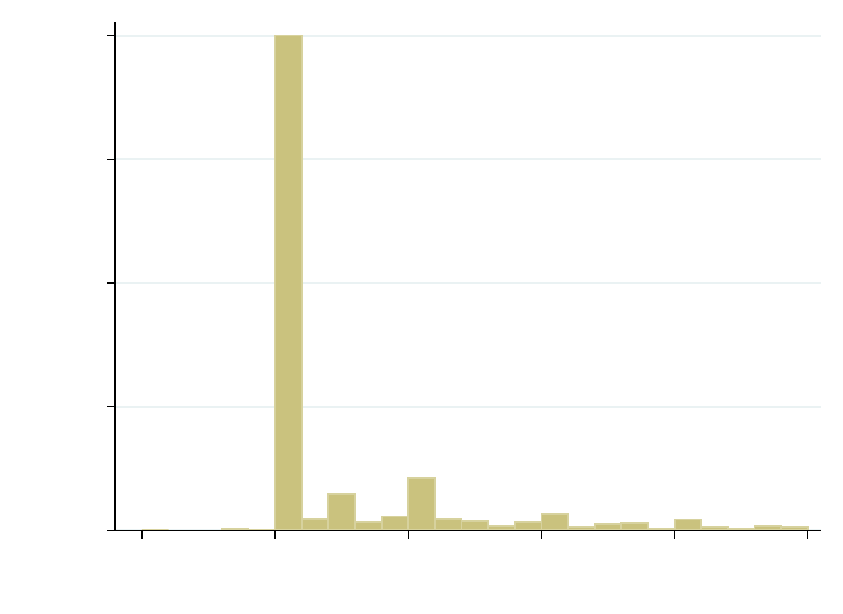
Appendix

0

20,000

40,000

60,000

80,000

0 .05 .1 .15 .2 .25

% Downpayment

Figure 8: Down payments of EL borrowers

The histogram shows data from the Help To Buy Equity Loan dataset from the UK Home and Communities

Agency (HCA). All EL borrowers who joined the scheme since its inception, in April 2013, to June 2016.

46

Table 7: Descriptive statistics: EL data

The table displays aggregate statistics for all Equity Loans issued between April 2013 and June 2016 in

England. Values are in British pounds.

Number of loans 91,759

Average purchase price 226,887

Average equity loan 45,442

Total value purchased properties 20,818,909,184

Total value equity loans 4,169,738,752

47

Table 8: Matching the data and constructing the estimation dataset

The table describes the sequential steps taken to construct the estimation sample. The dataset construction

has three parts. In the ﬁrst part, we open the universe of residential mortgage originations in the UK (the

Product Sales Data from the Financial Conduct Authority) and we restrict the sample to the period and

geographic area of interest, and we exclude mortgages for reﬁnancing purposes (remortgages). In the second

part, we match the data on Help To Buy Equity Loans (EL) from the Homes and Communities Agency into

the mortgage originations data. In the third part, we restrict the data to the EL group and the standard

mortgage group used in the main analysis of the paper; these include only mortgages on new build and with

a loan-to-value (LTV) ratio between 70 and 75%. (In practice we set the LTV limit at 76 because in the UK

mortgage fees are often rolled over into the principal, raising the measured LTV).

Sample Observations

1) Preparing mortgage originations data

Full Product Sales Data, 4/2005 - 3/2017 15,520,210

England only, 4/2013 - 3/2017 3,432,251

No remortgages 2,177,956

No duplicates in price, lender, date of birth, postcode, loan value 2,170,761

2) Matching EL data and mortgage originations data

Joinby 1 (full postcode, price, lender) 66,617

Drop duplicates and implausible matches 63,413

Joinby 2 (postcode district, price, lender) 16,290

Drop duplicates and implausible matches 9,179

Total matched (joinby 1 + joinby 2) 72,592

3) Bringing back matched loans into mortgage originations data; creating treatment and control groups

Loans with interest rate information 1,851,595

Only lenders doing EL mortgages 1,344,357

Only ﬁxed-rate mortgages with 2, 3, 5 or unknown ﬁxed period 1,151,455

Only new builds 185,604

Only properties with value below or equal to £600,000 180,886

Only LTVs between 70 and 76 69,832

Drop special mortgages, outliers, singletons 68,550

Drop if EL in London after January 2016 67,001

Drop if not EL and origination is after 30 June 2016 47,780

48