
fishR Vignette - Closed Mark-Recapture Abundance Estimates
Dr. Derek Ogle, Northland College December 16, 2013
The size of a population can be estimated by capturing and marking individuals from the population,
extracting another sample from the population at a later time, and determining the fraction of individuals in
the second sample that had the mark from the first sample. This idea was first used to estimate the population
of humans in London in 1662 (Krebs 1999), but was popularized in fisheries examinations by C.G.J. Petersen
in 1896 (Ricker 1975). The method was used by Lincoln (1930) for estimating duck populations and by
Jackson (1933) for estimating tsetse fly populations. Thus, this method is variously referred to as the
Petersen method, the Lincoln-Petersen method, or the Lincoln-Petersen-Jackson method. The “Petersen
method” will be used in this vignette.
The Petersen single-census method, which relies on only one sample of potentially marked fish, can be
extended to a series of samples. These extended methods, called the Schnabel and Schumacker-Eschmeyer
methods, require at least one sample where fish are marked and then multiple samples of potentially marked
fish. However, these methods are most often used when the unmarked fish in the subsequent samples are
marked and returned, along with the previously marked fish, to the population. Thus, these methods can
be used with multiple marking and multiple “recapturing” samples.
Use of the capture history form of data recording will be discussed in Section 1. The Petersen and related
methods are developed and implemented in Section 2 and the Schnabel and Schumacher-Escymeyer methods
are described in Section 3. This vignette requires functions in the FSA and FSAdata package maintained by
the author. These packages are loaded into R with
> library(FSA)
> library(FSAdata)
1 Individual Capture Histories
1.1 Data Format
For individually tagged fish, Pollock et al. (1990) recommended that the capture and recapture information
be recorded in the individual capture history format. In the individual capture history format, a data file
has as many rows as the number of unique fish that were observed at least once and as many columns as
sampling (or capture) periods. For each fish and sampling period cell of the file, a “0” is recorded if that
fish was not seen in that sample or a “1” is recorded if that fish was seen in that sample.
The capture histories for a hypothetical sample of four fish over five sampling periods is shown in Table 1.
For example, the first fish was captured in the first sample, not captured in the second sample, recaptured in
the third sample, and then not captured in either the fourth or fifth samples. The second fish was captured
in the first two samples and then not captured again. The fourth fish was not captured in the first four
samples and was captured for the first time in the fifth sample.
Table 1. Hypothetical example of the capture histories of four fish from five sample periods.
Sample Period
Fish 1 2 3 4 5
1 1 0 1 0 0
2 1 1 0 0 0
3 0 1 0 1 0
4 0 0 0 0 1
1

The capture histories considered in this vignette will only consist of “0”s and “1”s as discussed above.
However, more advanced applications will also use a “-1” for fish that were accidentally killed in the sampling
operation and were not returned to the population. For example, a capture history of (1, 0, −1, 0, 0) would be
recorded for a fish that was captured in the first sample and recaptured in the third sample but accidentally
killed before it could be returned to the population. The recording of accidentally killed specimens is
important as most multiple mark-recapture methods rely on knowing or estimating the number of extant
marks in the population. Recording that a fish was accidentally killed assures that it will not be included in
the number of extant marks.
Several subsequent analyses of the individual capture histories requires counting the frequency of individuals
with each capture history. These frequencies are typically symbolized with a lower-case “n” with the capture
history as a subscript. For example, n
10100
represents the number of fish that were captured in the first and
third sample periods but not in any other sample period.
This terminology can be extended to represent other frequencies by including a “dot” (i.e., ·) in the place
of any part of the subscript that is “summed across.” For example, n
··1··
represents the frequency of fish
that were captured in the third sample (i.e., a “1” in the third sample position) and either were or were not
captured in any of the other samples. In other words, n
··1··
represents the total number of fish captured in
the third sample. Traditionally, this value would also be referred to as n
3
where the subscript now represents
the sample number and not a capture history type. As another example, n
·101·
represents the number of
fish captured in the fourth sample that were last captured in the second sample. These and other specific
situations will have specific symbols in the context of specific methods later in this vignette.
1.2 Summarizing Capture Histories in R
A variety of useful summaries of capture history data can be obtained with capHistSum(). This function
requires a matrix or data frame that contains the raw capture history data. This matrix or data frame
must contain only the capture history data and no other data (e.g., a column with the fish identification
number must NOT be included). The cols= argument can be used to identify just the columns containing
the capture history information. For example, if the capture history information is contained in columns
two through seven then cols=2:7 should be used. Alternatively, if the capture history is contained in all
columns except for the first three then cols=-c(1:3) should be used. If the matrix or data frame contains
just the capture history information then the cols= argument can be ignored.
The capHistSum() function returns a list of four parts, the following two of which are used in this vignette:
caphist: A vector summarizing the frequency of fish with each unique capture history.
sum: A data frame containing the number of fish captured in each sample (n), the number of previously
marked fish captured in each sample (m), the number of marked fish returned to the population
following the sample (R), and the number of marked fish in the population just prior to the sample
(M). This summary is used in the Schnabel method for estimating population abundance (see Section
3).
The items in the list returned by capHistSum() can be individually accessed by assigning the results of the
function to an object and then appending the name of the item in the list to that object separated by a
dollar sign.
The use of capHistSum() is illustrated with the capture histories of northern pike (Esox lucius) from
Buckthorn Marsh that were recorded over four days in April by New York Power Authority (2004). The
individual capture histories were recorded in PikeNYPartial1 distributed in the FSAdata package which is
loaded with the FSA package. This data file is loaded into R and the structure observed with
> data(PikeNYPartial1)
> str(PikeNYPartial1)
data.frame : 57 obs. of 5 variables:
2

$ id : int 2001 2002 2003 2004 2005 2006 2007 2008 2009 2010 ...
$ first : int 1 1 1 1 1 1 1 1 1 1 ...
$ second: int 0 0 0 0 0 0 0 0 0 0 ...
$ third : int 0 0 0 0 0 0 0 0 0 0 ...
$ fourth: int 0 0 0 0 0 0 0 0 0 0 ...
The first six fish from the data frame are seen with
> head(PikeNYPartial1)
id first second third fourth
1 2001 1 0 0 0
2 2002 1 0 0 0
3 2003 1 0 0 0
4 2004 1 0 0 0
5 2005 1 0 0 0
6 2006 1 0 0 0
From this it is seen that the capture history information is contained in columns two through five, and that
the first column contains a unique fish identification number that should be ignored when summarizing the
capture histories. The capture history summaries for the capture history information recorded in columns
two through five is obtained with
> pikech1 <- capHistSum(PikeNYPartial1,cols=2:5)
The capture history summary and the Schnabel summary table can then be extracted with
> pikech1$caphist
0001 0010 0011 0100 0101 0110 1000 1001 1010 1100
5 8 2 12 1 2 21 1 2 3
> pikech1$sum
n m R M
1 27 0 27 0
2 18 3 18 27
3 14 4 14 42
4 9 4 0 52
Some researchers record capture history information in capture-by-event rather than in capture history
format. In capture-by-event format, each line of the data file contains the event (usually the date or sample
number) and the unique identification number for each captured fish. Capture-by-event format data should
be converted to capture history format data so that it can be efficiently summarized with capHistSum(). This
conversion is a rather complex process that is simplified with capHistConvert(). The capHistConvert()
function requires the data frame with the capture-by-event data as the first argument, the name of the
column containing the “events” in the event= argument, and the unique identification number in the id=
argument. In addition, if the event labels are characters, rather than numbers, then the correct order of the
level names should be included in the event.ord= argument.
The data in PikeNYPartial2 is the same as in PikeNYPartial1 except that it is recorded in capture-by-
event format. This data frame can be loaded into R and the structure and the first six individuals viewed
with
> data(PikeNYPartial2)
> str(PikeNYPartial2)
3

data.frame : 68 obs. of 2 variables:
$ sample: Factor w/ 4 levels "first","fourth",..: 1 1 1 1 1 1 1 1 1 1 ...
$ id : int 2001 2002 2003 2004 2005 2006 2007 2008 2009 2010 ...
> head(PikeNYPartial2)
sample id
1 first 2001
2 first 2002
3 first 2003
4 first 2004
5 first 2005
6 first 2006
From this it is seen that sample contains the events, id contains the unique identification number, and that
sample is a factor such that we will have to control the order of the events. With this information, the
conversion to capture history format is accomplished with
> PikeNYPartial2a <- capHistConvert(PikeNYPartial2,event="sample",id="id",
event.ord=c("first","second","third","fourth"))
> str(PikeNYPartial2a)
data.frame : 57 obs. of 5 variables:
$ id : Factor w/ 57 levels "2001","2002",..: 1 2 3 4 5 6 7 8 9 10 ...
$ Event1: int 1 1 1 1 1 1 1 1 1 1 ...
$ Event2: int 0 0 0 0 0 0 0 0 0 0 ...
$ Event3: int 0 0 0 0 0 0 0 0 0 0 ...
$ Event4: int 0 0 0 0 0 0 0 0 0 0 ...
> head(PikeNYPartial2a)
id Event1 Event2 Event3 Event4
1 2001 1 0 0 0
2 2002 1 0 0 0
3 2003 1 0 0 0
4 2004 1 0 0 0
5 2005 1 0 0 0
6 2006 1 0 0 0
The capture history summaries are then obtained with capHistSum() as
> pikech2 <- capHistSum(PikeNYPartial2a,cols=2:5)
> pikech2$caphist
0001 0010 0011 0100 0101 0110 1000 1001 1010 1100
5 8 2 12 1 2 21 1 2 3
The summaries returned by capHistSum() will allow for quick summarization of capture histories to be used
in the methods in Section 2 and Section 3.
2 Single Census Mark-Recapture Methods
2.1 Petersen Method
The Petersen method consists of two samples from a closed population and is, thus, the simplest of the
broad array of mark-recapture techniques for estimating animal abundance. The population and sampling
4
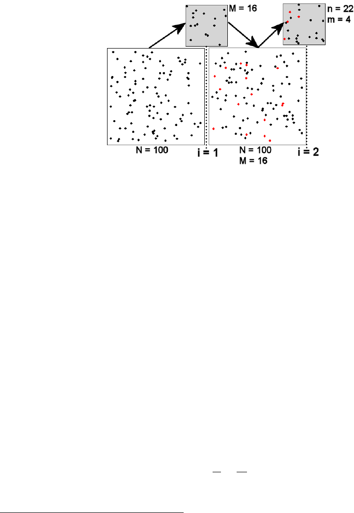
scheme for the two samples (i = 1, 2) of the Petersen method are represented in Figure 1. The large squares
just to the left of the “i=” vertical lines represent the population just before the ith sample is taken. The
large square just after the “i=1” vertical line represents the population just after the first sample was taken.
Thus, under the assumption that the population is closed, the population immediately after the first sample
is the same as the population immediately before the second sample. The samples are represented by the
small grey boxes just above each “i=” vertical line.
Figure 1. Schematic representation of the two samples (i = 1, 2) in a Petersen mark-recapture study. See
the text for detailed description and Table 3 for definitions of notation.
The population initially consists of all unmarked animals. All fish in the first sample are then marked
and returned to the population. The first sample does not necessarily need to be a random sample of the
population although the assumptions for the second sample are more likely to be met if it is. In addition,
the fish can receive a batch mark, i.e., each fish does not need to be uniquely identified
1
. The second sample
must be a random sample from the entire population of marked and unmarked individuals such that each
fish, whether marked or unmarked, has the same chance of being captured. This also implies that the marked
fish mix randomly with the unmarked fish in the population (Figure 1). Each fish in this second sample is
examined to determine if it has the mark from the first sample or not.
The summary data for a Petersen estimate can be shown in the format of capture histories (Table 2)
2
.
However, the more traditional notation of N = n
··
, M = n
1·
, n = n
·1
, and m = n
11
for ease of comparison
to other sources will be used throughout this vignette
3
. Remember that the capitalized symbols refer to the
population (i.e., N is number of fish in the population, M is the number of marked fish in the population)
whereas the lower-case letters refer to the second sample (i.e., n is the number of fish captured in the second
sample, m is the number of marked fish captured in the second sample). The meaning of the symbols used
in the Petersen method are shown in Table 3.
The Petersen estimate of abundance can be derived
4
from the initial assumption that if the second sample
is a random sample of the population of marked and unmarked animals, then the proportion of marked
animals in the second sample should equal the proportion of marked animals in the population, i.e.,
m
n
=
M
N
A rearrangement of this equality gives an estimate
5
of the size of the population, i.e.,
1
However, as mentioned in Section 1 it is generally beneficial to uniquely tag each fish.
2
An understanding of the notation used in capture histories is useful for using specialized computer programs indicated at
the end of the vignette.
3
The most traditional notation uses C = n
·1
, and R = n
11
. We do not use this notation in order to maintain continuity
with subsequent mark-recapture methods.
4
The Petersen estimate of abundance can also be derived from other starting points. Alternative derivations are shown in
Appendix A.
5
This re-arrangement derives a method-of-moments estimateor of N. This is also the maximum likelihood estimates as
5

Table 2. Summary data matrix for the two samples in a Petersen mark-recapture framework. Note that a
zero indicates the fish were not captured in that sample and a one indicates that the fish were captured in
that sample.
Second Sample
Not Captured (0) Captured (1) Total
First Not Captured (0) n
00
n
01
n
0·
Sample Captured (1) n
10
n
11
n
1·
Total n
·0
n
·1
n
··
Table 3. Summary of notation used in the Petersen method.
Symbol Meaning
N The unknown size of the population just prior to the first sample.
The number of fish from the first sample that were marked and
M
returned to the population.
n The number of fish in the second sample.
m The number of marked fish in the second sample.
b
N The estimated size of the population just prior to the first sample.
ˆ
N =
Mn
m
(1)
Thus, the total population size can be estimated from the number of marked animals, the number of animals
observed in the second sample, and the number of animals in the second sample that had the mark.
Approximate confidence intervals for N are often used
6
, with the specific form of the approximation de-
pending on characteristics of the number of marked and recaptured fish. Seber (1982) suggests the following
sequential “rules” (i.e., stop at the step where you answer “yes”) for choosing the method for approximating
the confidence interval for N in the Petersen method when sampling without replacement:
1. Is the fraction of marked fish in the second sample “large” (i.e.,
m
n
> 0.10)? – Use the binomial
approximation?
2. Is the number of marked fish in the second sample “large” (i.e., m > 50)? – Use the normal approxi-
mation?
3. Use the Poisson approximation.
Both the binomial and normal approximation methods identify a confidence interval for the ratio of marked
fish in the second sample (i.e.,
m
n
) and then the endpoints of these intervals are substituted into the modified
Petersen equation,
ˆ
N =
Mn
m
=
M
m
n
to derive endpoints of the confidence interval for N. The binomial approximation method constructs the in-
terval for
m
n
with computer algorithms of the binomial distribution. The normal approximation is considered
a large-sample method where the standard error for
m
n
is estimated with
shown in Appendix A.
6
Exact confidence intervals for N can generally be derived from the underlying distribution of the likelihood function (see
Appendix A). Unfortunately, there is no simple cumulative distribution for the hypergeometric distribution.
6

SE
m
n
=
s
1 −
m
M
m
n
1 −
m
n
n − 1
+
1
2n
The confidence interval is then constructed in the usual way with
m
n
± Z
∗
SE
m
n
.
The Poisson approximation operates similarly, except that it uses computer algorithms of the Poisson dis-
tribution to construct a confidence interval for m, the endpoints of which are then substituted back into (1)
to derive the confidence interval for N .
2.2 Modifications of the Petersen Method
The Petersen method of estimating abundance is the best asymptotically normal estimator as N approaches
infinity but, unfortunately, it is biased, especially for small samples. Chapman (1951) showed that when
M + n ≥ N that
ˆ
N =
(M + 1)(n + 1)
(m + 1)
− 1 (2)
is an exactly unbiased estimator of N
7
. If M + n < N, then Robson and Regier (1964) showed that the bias
of (2) is less than 2% if
Mn
N
> 4. Unfortunately, N is usually unknown. However, Robson and Regier (1964)
note that if m ≥ 7 then there is a 95% chance that
Mn
N
> 4 and the bias of (2) can be considered negligible
(Seber 1982). Thus, a given study should be designed so that enough fish are marked and the second sample
is large enough to ensure that more than seven marked fish are recaptured.
A final modification was proposed by Bailey (1951, 1952). Bailey’s method is appropriate if the second
sample of fish is collected with replacement (i.e., an individual may be counted more than once). This type
of sampling happens most often if the tagged fish are simply observed rather than captured. Bailey showed
that (1) is biased under these conditions and that his modified estimator,
ˆ
N =
(M)(n + 1)
(m + 1)
(3)
is nearly unbiased if m ≥ 7.
Confidence intervals for N from these modified estimators use techniques similar to those described for the
Petersen method. However, the binomial and normal confidence intervals for the ratio
m
n
must be converted
to a confidence interval for m by multiplying the endpoints by n. The endpoints of the confidence interval
for m are then substituted into (2) or (3) to obtain confidence intervals for N.
2.3 Petersen and Related Methods in R
The Petersen mark-recapture calculation can be made with mrClosed() with values of M , n, and m as the
first three arguments (in that order). The Chapman and Bailey methods can be used by changing the type=
argument in mrClosed() to "Chapman" or "Bailey", respectively. The results of this function should be
saved to an object so that point estimates and confidence intervals for N can be extracted with summary()
7
Ricker (1975) modified the Chapman estimator by ignoring the “-1” at the end of the right-hand-side of (2). His argument
was that subtracting one is of no practical importance in the estimate. While this argument is understandable, subtracting one
to get the exact result proposed by Chapman is not onerous. Therefore, we suggest using the full estimator as proposed by
Chapman (1951).
7

and confint(), respectively. The confidence intervals constructed by confint() will follow the suggestions
of Seber (1982)
8
. These methods will be illustrated for the following situation.
Concern over increases in the harvest of northern pike in Harding Lake prompted the Alaska Department
of Fish and Game to study this stock in 1990 (Burkholder 1991). One part of the study included capturing
northern pike, marking the fish with numbered floy tags and a partial pelvic fin clip, releasing the fish back
to the lake, and then recapturing these fish approximately one week later. The analysis only used northern
pike larger than 449 mm because of the selectivity of the gear used. The data were recorded in PikeHL and
can be loaded and viewed with
> data(PikeHL)
> head(PikeHL)
fish first second
1 1 1 0
2 2 1 0
3 3 1 0
4 4 1 0
5 5 1 0
6 6 1 0
The recorded capture histories, located in all but the first column of PikeHL, are then summarized with
> ch <- capHistSum(PikeHL,cols=-1)
> ch$caphist
01 10 11
135 297 49
These results show that there were M = 297 + 49 = 346 total fish captured, marked, and returned to the
population from the first sample, n = 135 + 49= 184 fish captured in the second sample, and m = 49
recaptured marked fish in the second sample. The population estimate, with corresponding confidence
interval, is then constructed with
9
> mr.p <- mrClosed(346,184,49)
> summary(mr.p)
Used the ’naive’ Petersen method with M=346, n=184, and m=49.
N
[1,] 1299
> confint(mr.p)
The binomial method was used.
95% LCI 95% UCI
[1,] 1034 1666
Thus, there appears to be between 1034 and 1666 northern pike in Harding Lake in 1990.
As an illustrative example, the estimated number of northern pike in Harding Lake in 1990 is computed
using the Chapman method with
8
The automatic choice of confidence interval type can be over-ridden, however, by including a specific method in the
type= argument to confint(). For example, to force calculation of confidence intervals with the binomial distribution use
type="binomial".
9
As a convenience, the object from capHistSum() can be sent solely to mrClosed() – i.e., mrClosed(ch) – to produce the
same results.
8

> mr.c <- mrClosed(346,184,49,type="Chapman")
> summary(mr.c)
Used Chapman’s modification of the Petersen method with M=346, n=184, and m=49.
N
[1,] 1283
> confint(mr.c)
The binomial method was used.
95% LCI 95% UCI
[1,] 1025 1636
2.4 Assumptions of Petersen & Related Methods
Before specifically adressing the assumptions of the Petersen and related methods it is important to note
that these estimates refer only to the catchable portion or the portion of the population fully recruited to the
gear. For example, if the population of northern pike studied was restricted to that part of the population
longer than 450 mm because of the gear used to capture the samples, then the estimates of abundance refer
only to that part of the population larger than 450 mm. In general, the population estimate only refers
to the population extant at the time of the first sample, except under very specific conditions which are
outlined below.
The Petersen and related methods depend on meeting five assumptions (Seber 1982):
1. The population is closed (so that N is constant).
2. All fish have the same chance of being caught in the second sample.
3. Tagging individuals does not affect their catchability.
4. Fish do not lose their tags between the first and second sample.
5. All tags are reported upon discovery in the second sample.
Fisheries personnel attempt to control the first assumption by having a very short period between the first
and second samples. However, there are several ways in which the first assumption can be violated without
adversely affecting the usability of the Petersen estimate (Seber 1982). If fish die while being marked and
before being released, then the Petersen estimate will refer to the size of the population after the marked
fish from the first sample are released. Mortality between the first and second sample will not affect the
Petersen estimate of initial population size if the rate of mortality is the same for both marked and unmarked
individuals (i.e., so the proportion of marked animals in the population is not affected). Recruitment of new
individuals to the population will completely invalidate the Petersen method as an estimator of the initial
population size. However, if there is no mortality along with the recruitment, then the Petersen method
will provide a valid estimate of the population size at the time of the second sample. Seber (1982) [p.73]
provides a statistical test to detect recruitment between the two samples.
The second assumption is difficult to assure because it is impossible to take a strict random sample in most
real situations. If all fish are equally catchable then a random sample can be approximated by sampling
areas at random with constant effort (Krebs 1999). Systematic sampling is often used to select animals but
this relies on the assumption that marked and unmarked animals mix uniformly through the population.
Unequal catchability between marked and unmarked fish may arise from three general causes (Eberhardt
1969):
1. The behavior of individuals in the vicinity of the trap.
9

2. Learning by animals already caught (i.e., trap-shy or trap-happiness).
3. Unequal opportunity to be caught because of trap positions.
Statistical tests exist (see Krebs (1999)) to identify certain forms of unequal catchability, but all of these
tests rely on more than two samples from the population. Thus, in a Petersen type study, the biologist must
take care to design fish collections that minimize these difficulties.
Finally, violations of the last two assumptions result in the possible underestimation of the proportion of
marked animals in the second sample which leads to overestimation of the population size. The fourth
assumption can be tested by “double-marking” a portion of the marked animals. For example, the northern
pike in Harding Lake were marked with a numbered floy tag and a partial fin-clip. The proportion of lost-tags
can be estimated from the recaptured fish and a correction applied to the population estimate.
3 Multiple Census Closed Population Mark-Recapture
3.1 Background
The population and sampling scheme for multiple sample methods on a closed population is shown in Figure
2. The setup of this figure is the same as that for the Petersen method (Figure 1), except that it is extended
for more than two samples. Note in this scheme that the population immediately after the ith sample is the
same as the population immediately before the (i + 1)th sample because the population is assumed closed.
For each sample period (i) a total of n
i
fish are captured. Each of the captured fish must be observed to
have a mark or not. The total number of marked fish in the ith sample is denoted with m
i
, whereas the
number of unmarked fish is u
i
. Immediately following the extraction of the ith sample, a total of R
i
marked
fish are returned to the population. The R
i
marked fish consists of the m
i
previously marked fish plus the
u
i
previously unmarked but now newly marked fish, minus any accidental deaths of fish captured in the
ith sample. The accidental deaths should be kept negligible as it is assumed, with these methods, that the
population is closed. Thus, R
i
is typically equal to m
i
+ u
i
. A summary of the notation used in these
methods is shown in Table 4.
Figure 2. Schematic representation of a hypothetical four samples (i = 1, 2, 3, 4) in a Schnabel or Shumacher-
Eschmeyer mark-recapture study. See the text for detailed description and Table 4 for definitions of notation.
The two multiple-sample closed population methods to be discussed also rely on determining the number of
marked fish extant in the population just prior to taking the ith sample, M
i
. Because these methods assume
a closed population, this task is as simple as accumulating the number of previously unmarked fish returned
to the population as marked fish prior to the ith sample. Thus, M
i
=
i−1
X
j=1
u
j
, or if there is the possibility of
10

Table 4. Summary of notation used in the Schnabel and Schumacher-Eschmeyer methods.
Symbol Meaning
N The unknown size of the population just prior to the first sample.
k The number of samples in the entire study (i.e., i = 1 . . . k)
n
i
The number of fish captured in the ith sample.
m
i
The number of marked fish in the ith sample. m
1
= 0
u
i
The number of unmarked fish in the ith sample.
The number of marked fish returned to the population after
R
i
the ith sample. R
k
= 0
The number of marked fish in the population just prior to
M
i
the ith sample. M
1
= 0
b
N The estimated size of the population just prior to the first sample.
some accidental deaths, M
i
=
i−1
X
j=1
(R
j
− m
j
). By definition, M
1
= 0 because there are no marked fish in the
population just prior to the first sample, .
These summary values – n
i
, m
i
, u
i
, R
i
, and M
i
– may be recorded directly from each sample or they may
be deciphered from summaries of individual capture histories. For example, suppose that the frequencies of
fish in each possible capture history is,
Capture history 001 010 011 100 101 110 111
Number of Fish 198 171 73 54 4 15 2
and there were no recorded accidental deaths. From this summary of capture histories, the required summary
statistics can be calculated. For example,
the number of fish captured in the first sample is
n
1
= n
1··
= n
100
+ n
101
+ n
110
+ n
111
= 54 + 4 + 15 + 2 = 75
the number of fish captured in the second sample is
n
2
= n
·1·
= n
010
+ n
011
+ n
110
+ n
111
= 171 + 73 + 15 + 2 = 261
the number of already marked fish captured in the second sample is
m
2
= n
11·
= n
110
+ n
111
= 15 + 2 = 17
the total number of marked fish released immediately after the first sample is
R
1
= m
1
+ u
1
− “accidental deaths” = 0 + 75 − 0 = 75
the total number of marked fish released immediately after the second sample is
R
2
= m
2
+ u
2
− “accidental deaths” = 17 + 244 − 0 = 261
the number of marked fish just before the second sample is taken
M
2
= M
1
+ (R
1
− m
1
) = 0 + (75 − 0) = 75
the number of marked fish just before the third sample is taken
M
3
= M
2
+ (R
2
− m
2
) = 75 + (261 − 17) = 319
11

These calculations, along with the remaining calculations not shown (i.e., n
3
and m
3
) and the default values
(m
1
= 0, R
3
= 0, and M
1
= 0), can be summarized in the following table,
ni mi Ri Mi
first 75 0 75 0
second 261 17 261 75
third 277 79 277 319
It should be noted that R
i
= n
i
only if there are no accidental deaths reported as was the case with this
example. Again, it is possible for R
i
< n
i
, but R
i
should not be substantially lower than n
i
.
3.2 Schnabel Method
The Schnabel equation for estimating N, derived in Appendix B, is
ˆ
N =
k
X
i=1
n
i
M
i
k
X
i=1
m
i
(4)
The Schnabel estimation formula is very similar in form to (1). In fact, Krebs (1999) noted that (4) is
basically a weighted average of individual Petersen estimates.
Chapman (1954) noted that (4) provides a slightly biased estimate of N . Therefore, he suggested that (4)
be modified with the inclusion of a 1 in the denominator,
ˆ
N =
k
X
i=1
n
i
M
i
k
X
i=1
m
i
!
+ 1
(5)
Krebs (1999) suggested that the Chapman modification of the Schnabel method should be used if the
proportion of the total population caught in each sample (i.e.,
n
i
ˆ
N
) is less than 0.1 and if the proportion of
the population that is marked (
M
i
ˆ
N
) is always less than 0.1. As a default, we suggest that the Chapman
modification should be used at all times.
Ricker (1975) and Krebs (1999) suggest two possible methods for constructing confidence intervals for N
with the Schnabel method. First, if
P
m
i
is small (i.e., < 50) then a Poisson approximation for constructing
a confidence interval for
P
m
i
is used and the endpoints substituted into (4) or (5) to construct confidence
endpoints for N (note that the confidence interval for
P
m
i
is constructed in the same manner as the
confidence interval for m in the Petersen method). Alternatively, when
P
m
i
is large then a confidence
interval is constructed for
1
N
using standard confidence interval methods and
SE
1
ˆ
N
=
v
u
u
u
u
u
u
u
u
t
k
X
i=1
m
i
k
X
i=1
n
i
M
i
!
2
with df = n − 2.
12

3.3 Schumacher-Eschmeyer Method
Schumacher and Eschmeyer (1943) provided a separate estimation function for N ,
ˆ
N =
k
X
i=1
n
i
M
2
i
k
X
i=1
m
i
M
i
(6)
that is based on minimizing the weighted sum-of-squares between the the proportion of marked animals in
a sample (i.e.,
m
i
n
i
) and the unknown proportion of marked animals in the population (the proof is given in
(Appendix C)).
The standard error of the reciprocal of this estimate is,
SE
1
ˆ
N
=
v
u
u
t
P
m
2
i
n
i
−
(
P
m
i
M
i
)
2
P
n
i
M
2
i
(k − 2)
P
n
i
M
2
i
where all of the summations extend from i = 1 to i = k and k is the number of samples. The confidence
interval for N is constructed by inverting the endpoints of the confidence interval for
1
N
computed as usual
with the standard error shown here.
3.4 Schnabel & Schumacher-Eschmeyer Methods in R
The mrClosed() function can be used to efficiently estimate N and construct associated confidence intervals
for the Schnabel method. The mrClosed() function is a flexible function that requires the n
i
and m
i
information and either the M
i
or R
i
information. If this summary information is already known, then it can
be sent as indivdual vectors in the n=, m=, M=, or R= arguments of mrClosed(). Alternatively this information
can be extracted from the sum component of the object saved from capHistSum(). Even more simply, if the
object from capHistSum() is sent as the first argument of mrClosed(), then the required information will be
automatically extracted. The Schnabel method is chosen by including type="Schnabel". Additionally, the
Chapman modification can be selected with the chapman.mod=TRUE argument (which is the default). The
results of this function should be saved to an object which can then be submitted to summary() to extract
the abundance estimate or confint() to extract the confidence interval for N . The use of this function is
illustrated in the following example.
The New York Power Authority conducted a detailed study of the Buckthorn Marsh Restoration Project area
to determine if the area was being used by northern pike as a spawning ground (New York Power Authority
2004). Part of the study included tagging age-1 and older pike captured in fyke nets and by electrofishing
with PIT tags and coded wire tags. The PIT tags were uniquely numbered and the CWT were used to assess
tag retention. Overall, fish were captured on 21 days between March 28 and May 2. The capture history of
the fish captured from April 1-4 are recorded in PikeNYPartial1. The data are loaded into R and viewed
with
> data(PikeNYPartial1)
> head(PikeNYPartial1)
id first second third fourth
1 2001 1 0 0 0
2 2002 1 0 0 0
3 2003 1 0 0 0
4 2004 1 0 0 0
13

5 2005 1 0 0 0
6 2006 1 0 0 0
From this it is seen that the captured histories are in all columns except for the first which contains the
unique fish identification numbers. Thus, the capture histories can be summarized using capHistSum() and
making sure to exclude the first column from the analysis, as such,
> ch1 <- capHistSum(PikeNYPartial1,cols=-1)
> ch1$sum
n m R M
1 27 0 27 0
2 18 3 18 27
3 14 4 14 42
4 9 4 0 52
The estimated number of northern pike in the Buckthorn Marsh Restoration Project, with 95% confidence
interval, is then estimated using the Chapman modification of the Schnabel method by with
> mr1 <- mrClosed(ch1,type="Schnabel")
> summary(mr1)
Used the Schnabel method with Chapman modification.
N
[1,] 128
> confint(mr1)
The Poisson method was used.
95% LCI 95% UCI
[1,] 75 238
Thus, there appears to be between 75 and 238 age-1 or older northern pike in Buckthorn Marsh.
To illustrate using mrClosed() with summary information, one can use the summary values for the complete
collection (not just the partial collection used above) of northern pike in the Buckthorn Marsh Restoration
Project (New York Power Authority 2004) found in PikeNY. These data are loaded and viewed with
> data(PikeNY)
> head(PikeNY)
date n m R
1 28-Mar 2 0 2
2 29-Mar 3 0 3
3 30-Mar 2 0 2
4 31-Mar 3 0 3
5 1-Apr 20 2 20
6 2-Apr 18 3 18
From this, one can see that the data file contains the n
i
, m
i
, and R
i
information in the n, m, and R variables.
Thus, the number of northern pike in the Buckthorn Marsh Restoration Project, with 95% confidence interval,
was estimated using the Chapman modification of the Schnabel method with
14

> mr2 <- with(PikeNY,mrClosed(n=n,m=m,R=R,type="Schnabel"))
> summary(mr2)
Used the Schnabel method with Chapman modification.
N
[1,] 87
> confint(mr2)
The normal method was used.
95% LCI 95% UCI
[1,] 71 113
Thus, there appears to be between 71 and 113 age-1 or older northern pike in Buckthorn Marsh.
The calculations of the Schumacher-Eschmeyer method can be made with mrClosed() by including the
type="Schumacher" argument. The other arguments are exactly the same as those described for the Schnabel
method except that the chapman.mod= argument is ignored. The number of northern pike in the Buckthorn
Marsh Restoration Project, with 95% confidence interval, was estimated using the Schumacher-Eschmeyer
method with
> mr3 <- with(PikeNY,mrClosed(n=n,m=m,R=R,type="Schumacher"))
> summary(mr3)
Used the Schumacher-Eschmeyer method.
N
[1,] 85
> confint(mr3)
The normal method was used.
95% LCI 95% UCI
[1,] 76 96
Thus, there appears to be between 76 and 96 age-1 or older northern pike in Buckthorn Marsh.
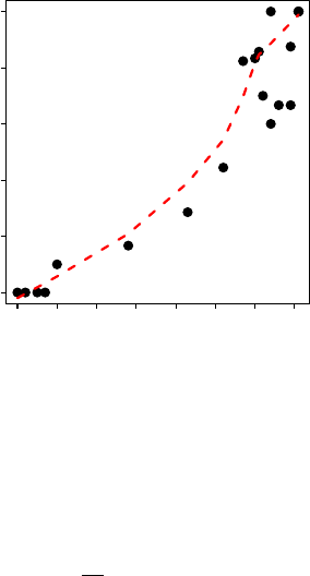
The plot of
m
i
n
i
against M
i
can be used to assess assumptions (see next section). This plot is constructed by
sending the object saved from mrClosed() to plot(). A loess smoother, which may help highlight curvature
in the plot, can be added to the plot by including the loess=TRUE argument. For example, the plot for the
entire collection of pike from Buckthorn Marsh (Figure ??) is constructed with
> plot(mr3,loess=TRUE)
It is clear from the curved nature of this plot that all of the assumptions for either the Schnabel or
Schumacher-Eschmeyer methods have not been met. Thus, the results shown in the previous two exam-
ples from these data should be interpreted with caution as they may be invalid.
3.5 Assumptions of Schnabel & Schumacher-Eschmeyer Methods
The Schnabel and Schumacher-Eschmeyer methods rest on the same assumptions as the Petersen method.
Thus, the discussion of the effect of violating assumptions of the Petersen method (see Section 2.4) pertains
15
0 10 20 30 40 50 60 70
0.0 0.2 0.4 0.6 0.8 1.0
M
i
m
i
÷ n
i
Figure 3. Plot of the proportion of marks in each sample versus the number of marked fish prior to the
sample for the Buckthorn Marsh Northern Pike dataset.
also to the Schnabel and Schumacher-Eschmeyer methods. One advantage of these multiple census methods
is that violations of the assumptions are more easily detected because of the multiple samples. The primary
diagnostic tool for these methods is the plot of
m
i
n
i
against M
i
. If this plot is not linear then one or more
of the assumptions of the Schnabel and Schumacher-Eschmeyer methods has been violated. Unfortunately,
the shape of the graph is not an indication of which assumption is violated (thus, the conclusion is that an
assumption has been violated but it is not clear which one).
References
Bailey, N. 1951. On estimating the size of mobile populations from capture-recapture data. Biometrika
38:293–306. 7
Bailey, N. T. J. 1952. Improvements in the interpretation of recapture data. Journal of Animal Ecology
21:120–127. 7
Burkholder, A. 1991. Abundance and composition of northern pike, Harding Lake, 1990. Fishery Data Series
91-9, Alaksa Department of Fish and Game. 8
Chapman, D. G. 1951. Some properties of the hypergeometric distribution with applications to zoological
censuses. University of California Publications on Statistics 1:131–160. 7
Chapman, D. G. 1954. The estimation of biological populations. Annals of Mathematics and Statistics 25:1–
15. 12
Eberhardt, L. L. 1969. Population estimates from recapture frequencies. Journal of Wildlife Management
33:28–39. 9
Feller, W. 1968. An Introduction to Probability Theory and its Applications, volume 1. Wiley, New York.
18
Jackson, C. H. N. 1933. On the true density of tsetse flies. Journal of Animal Ecology 2:204–209. 1
Krebs, C. J. 1999. Ecological Methodology. Second edition, Addison-Welsey Educational Publishing. 1, 9,
10, 12
Lincoln, F. C. 1930. Calculating waterfowl abundance on the basis of banding returns. U.S. Department of
Agriculture Circular 118:1–4. 1
16
New York Power Authority. 2004. Use of Buckhorn Marsh and Grand island tributaries by northern pike for
spawning and as a nursery. Technical report, New York Power Authority, niagara Power Project (FERC
No. 2216). 2, 13, 14
Pollock, K. H., J. D. Nichols, C. Brownie, and J. E. Hines. 1990. Statistical inference for capture-recapture
experiments. Wildlife Monographs 107:1–97. 1
Ricker, W. 1975. Computation and interpretation of biological statistics of fish populations. Technical Report
Bulletin 191, Bulletin of the Fisheries Research Board of Canada. 1, 7, 12
Robson, D. S. and H. A. Regier. 1964. Sample size in Petersen mark-recapture experiments. Transactions of
the American Fisheries Society 93:215–226. 7
Schnabel, Z. E. 1938. The estimation of the total fish population of a lake. American Mathematician Monthly
45:348–352. 20
Schumacher, F. X. and R. W. Eschmeyer. 1943. The estimation of fish populations in lakes and ponds.
Journal of the Tennessee Academy of Sciences 18:228–249. 13, 20
Seber, G. A. F. 1982. The Estimation of Animal Abundance. Second edition, Edward Arnold. 6, 7, 8, 9
Tuckwell, H. C. 1995. Elementary Applications of Probability Theory. 2nd edition, Chapman and Hall. 18
17

Appendices
A Petersen Abundance Estimate is MLE
Sampling Without Replacement
The Petersen method can also be cast as a Bernoulli process. After the marked fish are returned to the
population then the population consists of two types of fish – those that are marked and those that are
not. The removal of a single fish, which has probability
M
N
of being marked, and the recording of whether
it was marked (i.e., “success”) or not is the start of a Bernoulli process. If successive fish removed from the
population in the second sample are independent of each other then we have a true Bernoulli process and the
total number of marked fish found in the second sample (i.e., m) is a random variable that follows a binomial
distribution. If successive fish removed from the population in the second sample are not independent then
the total number of marked fish in the second sample follows a hypergeometric distribution. Strictly speaking,
the removal of the fish in the second sample are not independent, except in circumstances where the fish
are simply observed rather then removed in the second sample. However, if the population is large, the
number of marked fish is large, and the size of the second sample is relatively small then the assumption of
independent fish is not grossly violated and the binomial distribution may be used.
The likelihood functions for N can be constructed from the theory discussed in the previous paragraph. If
fish removed from the population in the second sample are not independent then the likelihood function
follows a hypergeometric distribution, i.e.,
L(N|M, n, n) =
M
m
N − M
n − m
N
n
(7)
The following is a proof, following that of Feller (1968) (as shown in Tuckwell (1995)), that the Petersen
estimate of abundance (i.e., (1)) maximizes this likelihood function.
This proof begins by creating the ratio of the likelihood function at two consecutive values of the population
size N, i.e., N and N − 1,
L(N|M, n, m)
L(N − 1|M, n, m)
=
M
m
N − M
n − m
N
n
M
m
N − 1 − M
n − m
N − 1
n
It is immediately seen that the first term in the numerators of both the numerator and denominator above
cancel. In addition, if the fraction in the denominator is flipped, multiplied times the numerator, and the
whole expression rearranged then the above expression, simplifies to,
L(N|M, n, m)
L(N − 1|M, n, m)
=
N − 1
n
N
n
•
N − M
n − m
N − M − 1
n − m
(8)
18

A fundamental property of combinatorics states that
A − 1
B
A
B
=
A − B
A
Thus, the two fractions in (8) can be simplified as,
L(N|M, n, m)
L(N − 1|M, n, m)
=
N − n
N
•
N − M
N − M − n + m
=
N
2
− N M − N n + Mn
N
2
− N M − N n + Nm
(9)
This ratio is equal to 1 if Mn = Nm or, equivalently, if N =
Mn
m
. In addition, the ratio is less than
1 if M n < Nm or N <
Mn
m
and is greater than 1 if Mn > N m or N >
Mn
m
. Therefore, the sequence
of L(N|M, n, m) for N = 1, 2, . . . is increasing when N <
Mn
m
and is decreasing when N >
Mn
m
and,
L(N|M, n, m) is maximized when N =
Mn
m
. This shows that the Petersen estimate of abundance (i.e., (1))
is a maximum likelihood estimator when the underlying distribution is hypergeometric.
Sampling With Replacement
Alternatively, as discussed in the previous section, if the fish removed can be considered independent then
the likelihood function follows a binomial distribution, i.e.,
L(N|M, n, m) =
n
m
M
N
m
1 −
M
N
n−m
(10)
The following is a proof that the Petersen estimate of abundance (i.e., (1)) maximizes this likelihood function.
This proof begins by noting that the combination in the binomial likelihood function (i.e., in (10)) does not
contain N and can, thus, be dropped from this maximizing procedure. Thus, the function to maximize is,
L(N|M, n, m) ∝
M
N
m
1 −
M
N
n−m
This is converted (and simplified) to a log-likelihood,
lnL(N |M, n, m) ∝ mln(M ) − N
1
log(N) + (n − m)log(N − M ) − (n − m)log(N )
∝ ml n(M ) + (n − m)log(N − M ) − nln(N )
The derivative of the log-likelihood with regard to N is (recall that the derivative for all terms in the
log-likelihood not involving N is zero),
∂lnL(N |M, n, m)
∂N
∝
n − m
N − M
−
n
N
This derivative is then set equal to zero and solved for N ,
19

n − m
N − M
−
n
N
= 0
n − m
N − M
=
n
N
Nn − N m = nN − nM
nM − N m = 0
N =
nM
m
Therefore, L(N |M, n, m) is maximized when N =
Mn
m
. This shows that the Petersen estimate of abundance
(i.e., (1)) is a maximum likelihood estimator when the underlying distribution is binomial.
B Schnabel Estimate of N
After the initial sample, the probability that a marked fish is captured is equal to the ratio of the number
of marked fish extant in the population to the size of the population (i.e.,
M
i
N
). Under the assumption
of sampling with replacement, the sampling process will be a Bernoulli process and the total number of
successes (i.e., marks) in a sample will follow a binomial distribution. Thus, the probability of observing m
i
marked and u
i
unmarked fish in the ith sample is given, by the binomial distribution, as
f(m
i
|M
i
, n
i
, m
i
) =
n
i
m
i
M
i
N
m
i
1 −
M
i
N
u
i
If the multiple samples are independent of each other then it follows that the likelihood function based on
the observed catches is
L(N|M
i
, n
i
, m
i
) =
k
Y
i=1
f(m
i
|M
i
, n
i
, m
i
) =
k
Y
i=1
n
i
m
i
M
i
N
m
i
1 −
M
i
N
u
i
This likelihood function is complicated, with k roots, but Schnabel (1938) showed that the positive real root
of
k
X
i=1
n
i
M
i
− m
i
N
N − M
i
(11)
is an approximate estimate of N. Furthermore, if M
i
is small relative to N then the denominator of (11)
is approximately N . Thus, after substituting N for N − M
i
in the denominator, straightforward algebraic
manipulation of (11) yields (4).
Schnabel (1938) also derived (4) beginning with a Poisson-based likelihood function and from an argument
based on the expected number of recaptures from a Poisson distribution.
C Schumacher-Eschmeyer Estimate of N
Schumacher and Eschmeyer (1943) noted that
ˆ
N is the value of N that minimizes the weighted least-squares
criterion,
20

L(N) =
k
X
i=1
n
i
m
i
n
i
−
M
i
N
2
(12)
The first step in this proof is to re-write (12),
L(N) =
k
X
i=1
n
i
m
2
i
n
2
i
− 2
m
i
M
i
n
i
N
+
M
2
i
N
2
=
k
X
i=1
m
2
i
n
i
− 2
m
i
M
i
N
+
n
i
M
2
i
N
2
The derivative of this function with respect to N yields,
∂L(N)
∂N
=
k
X
i=1
0 + 2
m
i
M
i
N
2
− 2
n
i
M
2
i
N
3
=
2
N
2
k
X
i=1
m
i
M
i
−
2
N
3
k
X
i=1
n
i
M
2
i
which is then set equal to 0 and N is solved for,
2
N
2
k
X
i=1
m
i
M
i
−
2
N
3
k
X
i=1
n
i
M
2
i
= 0
2
N
2
k
X
i=1
m
i
M
i
=
2
N
3
k
X
i=1
n
i
M
2
i
N =
k
X
i=1
n
i
M
2
i
k
X
i=1
m
i
M
i
21

Reproducibility Information
Version Information
Compiled Date: Mon Dec 16 2013
Compiled Time: 9:58:32 PM
Code Execution Time: 2.45 s
R Information
R Version: R version 3.0.2 (2013-09-25)
System: Windows, i386-w64-mingw32/i386 (32-bit)
Base Packages: base, datasets, graphics, grDevices, methods, stats, utils
Other Packages: FSA 0.4.3, FSAdata 0.1.4, gdata 2.13.2, knitr 1.5.15
Loaded-Only Packages: bitops 1.0-6, car 2.0-19, caTools 1.16, cluster 1.14.4, evaluate 0.5.1, for-
matR 0.10, Formula 1.1-1, gplots 2.12.1, grid 3.0.2, gtools 3.1.1, highr 0.3, Hmisc 3.13-0, KernSmooth 2.23-
10, lattice 0.20-24, MASS 7.3-29, multcomp 1.3-1, mvtnorm 0.9-9996, nlme 3.1-113, nnet 7.3-7, plotrix 3.5-
2, quantreg 5.05, sandwich 2.3-0, sciplot 1.1-0, SparseM 1.03, splines 3.0.2, stringr 0.6.2, survival 2.37-
4, tools 3.0.2, zoo 1.7-10
Required Packages: FSA, FSAdata and their dependencies (car, gdata, gplots, Hmisc, knitr, mult-
comp, nlme, plotrix, quantreg, sciplot)
22
