Can Zoning Reform Reduce Housing Costs? Evidence from Rents in Auckland

Can Zoning Reform Reduce Housing Costs? Evidence

from Rents in Auckland

Ryan Gree

naway-McGrevy and Yun So

arch 2024

Economic Policy Centre

WORKING PAPER NO. 016

Can Zoning Reform Reduce Housing Costs? Evidence

from Rents in Auckland

∗

Ryan Greenaway-McGrevy

†

and Yun So

‡

First version: May 2023 This version: March 2024

Abstract

Zoning reform is increasingly advocated to redress unaﬀordable housing, but there

are few real-world examples to demonstrate its eﬃcacy. However, in 2016, Auckland,

New Zealand, upzoned approximately three-quarters of its residential land, precip-

itating a boom in housing construction. In this paper we investigate whether the

zoning reform reduced housing costs, adopting a synthetic control method to spec-

ify rental prices in Auckland under the counterfactual of no zoning change. Rental

prices are measured using a hedonic index that quality-adjusts prices based on observ-

able attributes of the rental properties. Six years on from the reform, the synthetic

control from our preferred empirical speciﬁcation implies that rents would be approxi-

mately 28% higher under the counterfactual. This diﬀerence is statistically signiﬁcant

at a ﬁve percent level under the conventional rank permutation method applied to

post-treatment root mean squared error. Our ﬁndings support the proposition that

large-scale zoning reform can enhance housing aﬀordability.

∗

This research was funded by the Royal Society of New Zealand under Marsden Fund Grant UOA2013.

A previous version of this paper available here used the geometric mean of rents to measure rental

costs.Disclaimer: The results in this paper are not oﬃcial statistics. They have been created for re-

search purposes from the Integrated Data Infrastructure (IDI), managed by Statistics New Zealand. The

opinions, ﬁndings, recommendations, and conclusions expressed in this paper are those of the author(s), not

Statistics NZ, Ministry of Business, Innovation and Employment. Access to the anonymised data used in

this study was provided by Statistics NZ under the security and conﬁdentiality provisions of the Statistics

Act 1975. Only people authorised by the Statistics Act 1975 are allowed to see data about a particular

person, household, business, or organisation, and the results in this paper have been conﬁdentialised to

protect these groups from identiﬁcation and to keep their data safe. Careful consideration has been given to

the privacy, security, and conﬁdentiality issues associated with using administrative and survey data in the

IDI. Further details can be found in the Privacy impact assessment for the Integrated Data Infrastructure

available from www.stats.govt.nz. We would like to acknowledge the Public Policy Institute for providing

datalab access.

†

University of Auckland. Corresponding author. Postal address: The University of Auckland, Private

Bag 92019 Auckland 1142, New Zealand. Email: [email protected].

‡

Economic Policy Centre, University of Auckland.

1 Introduction

Housing has become increasingly expensive in many parts of the world, precipitating an

aﬀordability crisis (Wetzstein, 2017; Saiz, 2023). A large number of economists and urban

planners attribute unaﬀordable housing, at least in part, to restrictive zoning (Gyourko and

Molloy, 2015; Been, 2018; Hamilton, 2021). Zoning reform is consequently advocated to

reduce housing costs by relaxing regulatory restrictions on the supply of medium and high

density housing, such as plexes, rowhouses and apartments (Glaeser and Gyourko, 2003;

Freeman and Schuetz, 2017).

However, up until very recently, few cities have pursued

large-scale upzonings to enable aﬀordability (Schill, 2005; Freeman and Schuetz, 2017),

meaning there is little empirical evidence to support the posited eﬀects of zoning reform.

In particular, there is, as yet, no empirical evidence to support claims that large-scale

zoning reform can reduce the cost of housing.

However, in 2016 the city of Auckland, New Zealand, upzoned approximately three-

quarters of its residential land (Greenaway-McGrevy and Jones, 2023), precipitating a con-

struction boom in the city (Greenaway-McGrevy and Phillips, 2023; Greenaway-McGrevy,

2023a), and aﬀording us six years of data to examine the impact of the reform on housing

costs. In this paper, we assess the impact of the reform on rental prices, adopting a synthetic

control approach to specify the counterfactual scenario to the policy change. The synthetic

control is constructed from a donor pool comprising other commuting zones (which we

refer to as “urban areas”) in New Zealand, and matched to a variety of observed housing

market outcomes, including dwellings per capita and the average proportion of household

income allocated to housing among renting households. Rental prices are measured using

a hedonic price index constructed from individual dwelling data on rents available between

2000 and 2022.

Diﬀerences between actual and synthetic rental price indexes measure the impact of the

reform. However, the magnitude of the estimated policy impact is somewhat sensitive to

model speciﬁcation. Our baseline speciﬁcation implies that rents are 26.1% lower by 2022,

or, equivalently, rents would be 35.4% percent higher in Auckland under the counterfactual

of no reform (since 0.354 = 0.261/(1 − 0.261)). One particular donor unit receives a

weight of over seventy percent in this speciﬁcation. When this unit is omitted from the

donor set, the estimated decrease in rents falls to 21.6%, indicating that the ﬁndings from

the baseline model are highly dependent on the speciﬁc donor. To be conservative in

our assessment of policy eﬀects, we select a model speciﬁcation that omits this donor as

our preferred model. Thus, our preferred empirical speciﬁcation implies that rents in 2022

“Plexes” refers to duplexes, triplexes, sixplexes, etc.

At the time of writing, data were available for the years 2000 through 2022. We anticipate updating

the paper once data for 2023 become available.

would be 27.6% percent higher had Auckland not implemented zoning reform in 2016 (since

0.276 = 0.216/(1 − 0.216))).

The ﬁnding that large-scale zoning reform can reduce housing costs is important. While

researchers and policymakers have advocated for large-scale zoning reform as a means to

increase supply and enhance aﬀordability, studies that focus on localized (or “spot”) upzon-

ings typically show muted or no eﬀects on housing supply and/or aﬀordability (Freemark,

2020; Dong, 2021), casting doubt on the ability of zoning changes to meet intended ob-

jectives (Rodr´ıguez-Pose and Storper, 2020). Such studies are also misused by advocates

and policymakers opposed to zoning reform as evidence that large-scale reforms will fail

(Cheung et al., 2023). Recently, Stacy et al. (2023) examine over ﬁfty upzonings in various

cities in the U.S., ﬁnding only small eﬀects on housing construction and costs. Results

from the present synthetic control approach indicate that the zoning reform undertaken as

part of the Auckland Unitary Plan did enhance housing aﬀord ability, when measured by

rents, suggesting that large-scale reforms have substantially diﬀerent impacts to localized

upzonings. This should be unsurprising. Compared to large-scale upzoning, conferring

redevelopment rights to a limited number of locations reduces the number of development

opportunities, and consequently generates less housing supply and smaller eﬀects on hous-

ing costs.

Rental price indexes are constructed using the Ministry of Housing and Urban Devel-

opment (MHUD) dataset on individual rental bonds, which reports the weekly rent on new

tenancies in the country. The dataset also includes information on the number of bed-

rooms, property type (house, apartment or ﬂat), state or private ownership, and location

(by meshblock). From these data, we calculate imputed hedonic price indexes using new

tenancies within each commuting zone. The price indexes are therefore quality-adjusted

using the observable attributes of the tenancies, including the number of bedrooms, housing

type, and location.

We use rents, rather than house prices, to measure housing costs for two reasons. First,

rents are not directly aﬀected by enhanced redevelopment rights from zoning reform. The

eﬀects of upzoning on housing prices is mediated by the land endowment of aﬀected prop-

erties. Land prices in desirable locations increase in value (Greenaway-McGrevy, 2023b),

reﬂecting the increased capacity of the land to hold additional ﬂoorspace and the right to

redevelop the property into capital intensive dwellings. Properties that are relatively land

intensive, such as detached single family dwellings on large lots, are likely to appreciate in

value. Greenaway-McGrevy et al. (2021) present evidence consistent with this reasoning

after the reforms in Auckland. Rents, on the other hand, are not aﬀected by the enhanced

development rights, which accrue to the landowner. Second, rents potentially capture hous-

ing costs across a wider socioeconomic demographic, given that low income households are

more likely to be tenants.

To assess the statistical signiﬁcance of estimated rent decreases, we apply the rank

permutation test to the post-intervention root mean square errors (RMSEs) when the

placebo interventions are applied to donor units. Auckland has the largest post-treatment

RMSE among all 49 units in the donor pool, indicating that the counterfactual does a poor

job of describing actual outcomes, as would be anticipated if the policy was eﬀective. If one

were to assign the intervention at random, the probability of obtaining a ratio as large as

Auckland’s is at most 0.02 (= 1/50). However, applying the rank permutation test to the

ratio of post- to pre- intervention RMSEs (Abadie et al. 2010), Auckland ranks between

third and twelfth, depending on model speciﬁcation.

The synthetic control method has been applied to evaluate policy in a variety of contexts

(see Abadie, 2021 for a comprehensive review). We take several steps to ensure that our

research design and implementation is robust to common pathologies. First, we use the

longest possible times series on outcomes prior to intervention in order to minimize bias in

the synthetic unit (Abadie et al., 2010). Our rental time series spans 2000, when data for

individual bond tenancies begin, to 2022, with the intervention occurring in 2016. Second,

we examine how robust our ﬁndings are to changes in modeling assumptions, including

changes in the viable units in the donor set. Although the magnitude of implied rent

decreases does vary somewhat between speciﬁcations, in all speciﬁcations the decreases

are substantial. Third, our ﬁndings are largely unchanged under conventional robustness

check exercises that are commonly adopted in the synthetic control literature, including

the “leave one out” robustness check (Abadie et al., 2010), whereby units from the donor

pool are iteratively removed from the sample while the procedure is repeated.

Nonetheless, there are inherent limitations to the synthetic control method. Donor

units will be aﬀected by the policy intervention if increased housing supply in Auckland

aﬀects inter-city migration of tenants. Note, however, that in-migration to Auckland due

to lower housing costs generates attenuation bias in estimates of the casual impact, since

it reduces housing demand in other cities. More problematic is a population decrease in

Auckland from 2020 onwards, widely attributed to COVID-19 and policy responses thereto.

Statistics New Zealand estimates that Auckland’s population decreased by 1.1% between

June 2020 and June 2022, before increasing by 2.4% between June 2022 and June 2023.

Although media attention at the time focused mainly on Auckland, the same population

estimates show that other cities experienced population decreases between 2020 and 2022,

including (but not limited to) Dunedin (1.79%), Wellington (0.14%) and Rotorua (0.4%).

Notably, these cities experienced signiﬁcant appreciation in rents between 2020 and 2022,

despite population decreases. We address this problem in two ways. First, we end the

sample in 2020, when the estimates of Auckland’s population peak. Rents in Auckland are

17.3% less than those of the synthetic control at this point. Second, we include estimates of

population decrease between 2020 and 2022 in the set of matching variables, and drastically

reduce the set of matching variables to those that feasibly predict the exodus, so that the

population decrease variable plays a prominent role in constructing the synthetic control

for Auckland. Rents are 22.9% less than those of the synthetic control in this speciﬁcation

– a larger decrease than that obtained under our preferred speciﬁcation.

The remainder of the paper is organized as follows. The following section provides

the institutional details of the policy and provides a general background on Auckland and

New Zealand. Section three describes the data. In section four presents the method and

results. We ﬁrst present our baseline empirical speciﬁcation, before exploring variations of

the baseline model. Section ﬁve concludes.

2 Institutional Background

Housing costs in New Zealand are among the most expensive in the developed world.

Among renters and owner-occupiers with a mortgage, the median proportion of disposable

income (i.e. after taxes and transfers) spent on housing costs was 22% in 2021, exceeded

only by Australia, Greece and France in the OECD.

Among renting households, the median

proportion is 28%. As of the 2018 census, over a third (35.5%) of households are tenants.

This ﬁgure is higher for Auckland, where more than two-ﬁfths (40.6%) of households rent

as of 2018.

Auckland is the largest city in New Zealand, with a population of 1.57 million as of

2018 (source: New Zealand census). In March 2013, the city announced the ﬁrst version

of the Auckland Unitary Plan (AUP), which introduced and applied a standardized set

of planning zones across the jurisdiction, including four new residential zones. Three of

these zones encourage various gradations of medium to high density housing. After several

rounds of reviews and consultation, the plan was made operative in November 2016. Ap-

proximately three-quarters of residential land was upzoned, in the sense that eﬀective FAR

restrictions on housing development were relaxed (Greenaway-McGrevy and Jones, 2023).

For additional details on the implementation of the plan and the spatial distribution of

upzoning, see Greenaway-McGrevy and Jones (2023).

Although the plan was operationalized in 2016, an agreement between the Auckland

Council and the central government called the ’Auckland Housing Accord’ allowed devel-

See Figure 10 here: https://www.msd.govt.nz/documents/about-msd-and-our-work/

publications-resources/monitoring/household-income-report/2021/international-

comparisons-of-housing-affordability.docx. Data for Auckland is not available.

Source: 2018 census https://www.stats.govt.nz/tools/2018-census-place-summaries/

auckland-region#housing

Figure 1: New dwelling permits in Auckland by 2016 zoning reform, 2000 to 2022

2000 2002 2004 2006 2008 2010 2012 2014 2016 2018 2020 2022

New dwelling permits (thousands)

Reform

Partial Reform

Non-Upzoned Residential, Business and Rural Areas

Upzoned Residential and Business Areas

Notes: New dwelling permits in areas that were upzoned and were not upzoned in 2016 under the AUP.

The ﬁrst, “draft”, version of the AUP was announced in March 2013, while the “Proposed” AUP (PAUP)

was notiﬁed in September 2013. Partial zoning reform was implemented in early October 2013 under the

Auckland Housing Accord. Between October 2013 and November 2016, Special Housing Area (SpHA)

developments could build to the regulations of the PAUP in exchange for aﬀordable housing provisions.

Full reform occurred in November 2016 when the ﬁnal version of the AUP became operative. Source:

Greenaway-McGrevy (2023a).

opers to build to the rules of the ’Proposed’ Auckland Unitary Plan (PAUP), announced

in September 2013.

This was an inclusionary zoning program that required developers to

oﬀer a 10% proportion of aﬀordable housing in exchange for accelerated permitting process

and the ability to build to the more relaxed land use regulations under the PAUP.

The

program ended once the AUP was implemented.

Housing supply quickly responded once the AUP was operative in 2016. Figure 1 ex-

hibits new dwelling permits issued per year, decomposed into upzoned and non-upzoned

areas. Permits increased signiﬁcantly year-on-year from 2016 onwards, after the AUP is

operative, with all of the new construction occurring in upzoned areas. There is some

limited evidence of divergence from 2013 onwards, reﬂecting policy “leakage” as some de-

velopers took advantage of the relaxed regulations under the PAUP (see Figure 11 in the

Appendix, which separately identiﬁes PAUP-SpHA permits in the data). Nonetheless, we

use 2016 as the date of the policy intervention in the synthetic control exercise, since this

the date after which the divergence becomes most evident, and accords with the full reform

becoming operative.

Our outcome of interest – rents – are likely to have been impacted by several legislative

changes over the period of analysis. However, these changes aﬀected rental housing across

See https://www.beehive.govt.nz/sites/default/files/Auckland_Housing_Accord.pdf

The “Housing Accords and Special Housing Areas Act 2013” (HASHAA). See https://www.

legislation.govt.nz/act/public/2013/0072/latest/DLM5369001.html

the whole country, and we have little reason to think these changes would have a dispro-

portionate eﬀect on Auckland. The sixth Labour government (2017–2023) substantially

altered regulations governing tenancies and the taxation of housing investors. Beginning

in 2018, it introduced a series of bills to: protect and enhance renters’ rights, including the

prohibition of letting fees and bidding for tenancies; limit tenant liabilities; and restrict

rent price increases (to every twelve months) and cause to terminate tenancies.

Legis-

lation to enhance minimum health and safety standards was passed in July 2019.

Tax

treatment of property investment also changed. From April 1, 2019, landlords could no

longer oﬀset property investment losses against other sources of income when calculating

their income tax liability (known as ‘ring-fencing’),

and their ability to claim mortgage

interest as an expense on the rental property was phased out from October 2021.

Our

sample period also spans recent demand-side policies intended to curb housing demand

to promote house price aﬀordability, including severe restrictions on foreign ownership,

disincentives to investor speculation, and macroprudential banking restrictions.

These

changes aﬀected houses in all urban areas of the country, but nonetheless underscore the

need for the informed selection of a counterfactual scenario for policy evaluation.

3 Data

Individual data on new tenancies are collected by the Ministry of Housing and Urban De-

velopment (MHUD) on a quarterly basis. The data are not public, but can be accessed

via Statistics New Zealand’s Integrated Data Infrastructure (IDI). In addition to the rental

price, the dataset contains information on the rental property, including the number of bed-

rooms, housing types (“Flats” and “Houses”), public or private ownership, and meshblock,

which are equivalent to census tracts in the U.S. and provide a measure of location. From

these data we construct hedonic imputation price indexes, using number of bedrooms,

and indicators apartment, ﬂat, and location (speciﬁcally, statistical area 2 units, which

comprise meshblocks).

We use the “double” imputation method, whereby the hedonic

regression is used to estimate prices in both the period of transaction and the period prior

See https://www.legislation.govt.nz/act/public/2018/0044/latest/LMS24553.html,

https://www.legislation.govt.nz/act/public/2020/0059/latest/LMS294929.html and https:

//www.legislation.govt.nz/act/public/2019/0037/latest/DLM7247512.html

Known as the “Healthy Homes Standards”. See https://www.legislation.govt.nz/regulation/

public/2019/0088/latest/whole.html.

See https://www.legislation.govt.nz/act/public/2007/0097/486.0/LMS223653.html

See https://www.legislation.govt.nz/act/public/2007/0097/latest/LMS675468.html

Loan to value ratios on new residential mortgages were introduced in 2013; a capital gains tax based

on duration of ownership was introduced in 2015; and legislation preventing foreign ownership (excepting

Australia and Singapore) in 2018. See Greenaway-McGrevy and Phillips (2021) for additional details.

We use ﬁxed eﬀects at the larger statistical area 2 (SA2) level, rather than meshblocks, due to data

sparsity at higher geographic resolutions. SA2s contain 2,000 to 4,000 persons in urban areas.

to the transaction (Eurostat, 2013). Refer to the appendix for a detailed description of the

method.

We use hedonic imputation to measure rental price changes because dwellings are het-

erogenous and infrequently transacted. Hedonic methods are more appropriate for diﬀeren-

tiated products or services (Silver and Heravi, 2007) than common alternatives such as re-

peated transaction (matched model) methods. For instance, repeated transaction methods

are subject to the “new goods” problem (Pakes, 2003), which refers to distortions in price

measurement stemming from changes in the composition of diﬀerentiated products within

the broader product class over time. Price diﬀerentials between diﬀerent products are not

used in the measurement of inﬂation, which becomes problematic when new products are

introduced and extant products are retired each period. The problem is particularly acute

in housing, as each dwelling is diﬀerent and infrequently transacted. Repeated transaction

methods are also subject to the “lemon’s bias” when applied to housing, because measured

prices become biased towards more frequently transacted properties (Clapp and Giaccotto,

1992).

Among the diﬀerent hedonic approaches, hedonic imputation oﬀers greater ﬂexibility

than the hedonic time dummy approach, as it allows the hedonic coeﬃcients on product

or service attributes to change over time. Pakes (2003) advocates for the use of hedonic

imputation over time dummy methods “since hedonic coeﬃcients vary across periods it

[the time dummy hedonic method] has no theoretical justiﬁcation.” Hedonic imputation

methods are generally preferred by statistical agencies such as Eurostat when measuring

house prices (Eurostat, 2013, pp. 159).

We use Functional Urban Areas (FUAs) as the geographic units of analysis. FUAs

are delineated by Statistics New Zealand on the basis of commuting patterns, and are

analogous to commuting zones as deﬁned by the OECD.

There are 53 FUAs in New

Zealand, including Auckland. Henceforth, we use “urban areas” (UAs) as shorthand for

FUAs.

Figure 2 exhibits the rental price indexes for Auckland and the other urban areas of

New Zealand. Indexes are normalized to one in 2016, the year in which the zoning reform

becomes operational. We include a population-weighted average of the other urban areas.

Over the decade prior to the reform, rents in Auckland are growing at a faster rate

A previous version of this paper available here used the geometric mean of rents to measure rental

costs. As discussed in that version, a drawback of using averages (as opposed to quality-adjusted price

indexes) is that systematic changes in the composition of the rental stock can manifest as price changes.

Statistics New Zealand produces rental price indexes for ﬁve regions using a time dummy hedonic

model that is ﬁtted to individual rental bond data over an eight-year sample window (see Bentley, 2022).

Because the model includes individual dwelling ﬁxed eﬀects, rental price changes are inferred from repeated

tenancies within the sample window, and are therefore subject to the new goods problem and lemon’s bias.

See https://www.stats.govt.nz/assets/Methods/Functional-urban-areas-methodology-and-

classification.pdf

that in the rest of the country (the rental price index is higher than the Auckland index

between 2007 and 2014 or so). In the six years since the reform, rental price increases in

the other urban areas have far exceed those in Auckland. By 2022, the rental price index

in Auckland is 1.181, whereas the population-weighted price index is 1.513. Rental prices

in other urban areas (as measured by the population-weighted average) have increased by

33.2 percentage points relative to Auckland between 2016 and 2022. This is a substantial

divergence.

Figure 2 also presents the index for Auckland against other the “metropolitan” urban

areas of the North Island of New Zealand: Auckland, Hamilton, Tauranga and Wellington.

We select these three urban areas as they are large cities that are comparatively close to

Auckland. (This comparison is purely for expositional purposes: In the analysis to follow we

use the synthetic control method to select appropriate controls.) Prior to the reform, rental

prices in Auckland were growing at a faster rate than in Hamilton and Wellington, but at

a slower rate than Tauranga. After the reforms, rental prices in Auckland are growing at a

slower rate than all three cities. By 2022, the rental price indexes of Tauranga, Hamilton

and Wellington range between 1.396 to 1.434. Thus, between 2016 and 2022, rental prices

in the other metropolitan cities of the North Island increased by 21.5 to 24.3 percentage

points more than Auckland. In other words, the inﬂation rate in Auckland after the AUP

was approximately half of that of proximate metropolitan cities.

3.1 Matching Variables

As we demonstrate in more detail in the following section, the synthetic control method

selects comparable control units by matching outcomes prior to the policy intervention.

These can include the outcome of interest (in our application, rental price indexes) as

well as other related variables. Here we describe the additional matching variables, all of

which are housing market outcomes, determinants of outcomes, or exogenous constraints

on housing supply.

Population growth. This is the log diﬀerence of estimated population by FUA. Censuses

occur in 2001, 2006, 2013 in the pre-reform era.

Dwellings per capita. This is the number of occupied dwellings in the FUA divided by

the usually resident population in the FUA. Both ﬁgures are obtained from census data.

The measure is obtained for the pre-reform census years of 2001, 2006, and 2013.

Statistics NZ classiﬁes urban areas as either “metropolitan”, “large”, “medium” or “small”.

Figure 2: Rental price indexes in urban areas, 2000–2022

2000 2002 2004 2006 2008 2010 2012 2014 2016 2018 2020 2022

Year

0.4

0.6

0.8

1.2

1.4

1.6

1.8

2.2

2.4

Rent Price Index (2016 = 1)

Reform

Auckland

Population-Weighted Average of Other Urban Areas

Other Urban Areas

2000 2002 2004 2006 2008 2010 2012 2014 2016 2018 2020 2022

Year

0.4

0.6

0.8

1.2

1.4

1.6

Rent Price Index (2016 = 1)

Reform

Auckland

Hamilton

Tauranga

Wellington

Notes: Rental price indexes for Auckland and other urban areas of New Zealand, 2000 to 2022. Population

weights based on 2018 census populations. Indexes normalized to one in 2016, the year of Auckland’s

reform.

Personal income. We obtain the average personal income (from all sources) for the

census years 2001, 2006 and 2013 by FUA from Statistics New Zealand.

Proportion of renting households. Proportion of renting households within the FUA

for the two census years prior to the intervention, 2006 and 2013, by FUA from Statistics

New Zealand. Data for earlier census years for the required geographic units is unavailable.

Share of housing costs for renting households. We include the average proportion

of household income spent of rental costs for renting households, for 2006 and 2013. Census

data obtained from Statistics New Zealand. Data for earlier census years for the required

geographic units is unavailable.

Developable land. We calculate the proportion of the area within 25 kilometers of the

center of the urban area that is land under a 10 degree slope. We take the location of the

local council oﬃce as the center. This measure is inspired by Saiz (2010), who uses land

under a 15% slope as an exogenous instrument for housing supply, as such land can be

easily developed.

4 Synthetic Control Method and Results

This section outlines the synthetic control method and applies it to our dataset.

4.1 Synthetic Control Method

We have time series data on an outcome of interest for N +1 units indexed by i = 1, ..., N+1,

where i = 1 corresponds to the unit receiving the policy intervention, and i = 2, ...., N + 1

indexes the “donor pool”, a collection of untreated units that are unaﬀected by the inter-

vention.

Observations on the outcome of interest span t = 1, ..., T , where the observations

prior to intervention span t = 1, ..., T

and T

< T − 1.

i,t

denotes the observed outcome of interest for unit i in period t. A synthetic control

is deﬁned as a weighted average of the units in the donor pool. Given a set of weights

w = (w

, ..., w

N+1

), the synthetic control estimator of y

1,t

is ˆy

1,t

N+1

i=2

i,t

. Let y

1,t

the (unobservable) outcome without intervention for the ﬁrst unit, while y

1,t

is the outcome

under the intervention in period t > T

. The eﬀect of the intervention is then y

1,t

− ˆy

1,t

Abadie and Gardeazabal (2003) and Abadie et al. (2010) choose w so that the resulting

synthetic control best resembles a set of pre-intervention “predictors” for the treated unit.

This section borrows heavily from Greenaway-McGrevy (2023a).

For each i, there is a set of k observed predictors of y

i,t

contained in the vector X

1,i

, ..., x

k,i

), which can include pre-intervention values of y

i,t

unaﬀected by the intervention.

The k × N matrix X

= [X

· · · X

N+1

] collects the values of the predictors for the N

untreated units. Abadie and Gardeazabal (2003) and Abadie et al. (2010) select weights

∗

= (w

∗

, ..., w

∗

N+1

) that minimize

∥X

− X

w∥

h=1

h,1

− w

h,2

− ... − w

N+1

h,N+1

)

1/2

(1)

subject to the restrictions w

∈ [0, 1] and

N+1

i=2

= 1, and where v = (v

, ..., v

) is a set

of non-negative constants. Following Abadie et al. (2010), we choose v to assign weights to

linear combinations of the variables in X

and X

that minimize the mean square error of

the synthetic control estimator in the pre-treatment period. Then, the estimated treatment

eﬀect for the treated unit at time t = T

, . . . , T is ˆy

1,t

N+1

i=2

∗

i,t

Weights w that minimize (1) can found using standard quadratic programming solvers.

To select v in the nested RMSE-minimization problem, we use Evolution Strategy with

Covariance Matrix Adaptation (CMA-ES), which is a stochastic optimization algorithm

for solving diﬃcult optimization problems (Hansen, 2016). It is considered a state of the

art evolutionary optimizer (Li et al., 2020).

In our application, we include all pre-treatment realizations of the outcome variable,

rents, in the set of predictors. As discussed in Abadie et al. (2010) and Abadie (2021),

increasing the pre-intervention time period T

reduces the bias in the synthetic control. In

our baseline speciﬁcation, we include rents between 2000 and 2016. As discussed above,

we also include dwellings per capita, the proportion of renting households, and average

proportion of household income spent on rent among the matching variables. See section

three above for a discussion of the rationale for including these variables.

The synthetic control requires that the predictors of the treated unit must lie within the

convex hull of the predictors of the donor pool. The convex hull assumption is necessary

for the treated unit’s predictors to be approximated by the donor pool’s. We normalize the

price indexes to be one in 2016, and then take logs. Auckland’s price index satisﬁes the

convex hull condition prior to treatment.

We employ a hierarchical restriction of the donor pool for each urban area based on

Statistics New Zealand categories. Urban areas (UAs) in New Zealand are categorized as

“metropolitan”, “large”, “medium” and “small”, depending on size. “Metropolitan” con-

sists of six cities; “large” consists of eleven; and “medium” a further fourteen. The remain-

We adapt the Matlab version of the Synth package provided by Jens Hainmueller (available from

https://web.stanford.edu/

jhain/synthpage.html) to incorporate CMA-ES minimization of nested

RMSE objective function, using the cmaes.m matlab code provided by Nikolaus Hansen (available from

http://cma.gforge.inria.fr/cmaes.m).

der are “small”. Metropolitan UAs have their donor pool restricted to other metropolitan

UAs and large UAs in order to encourage similarity between Auckland its potential donors.

Abadie (2021, p. 409) notes that restricting the donor pool to units with similar charac-

teristics to the treated unit helps minimize interpolation biases. For placebo tests, large

UAs have their donor pool restricted to metropolitan, large and medium UAs. Medium

and small UAs do not have their donor sets restricted.

We omit Christchurch from the donor pool due to the impact of the 2011 earthquake

on its housing stock and other housing outcomes. As noted by Abadie (2021) (p. 409),

potential donor units that are subject to large idiosyncratic shocks to the outcome variable

should be withheld from the donor set. We also omit Queenstown, where rents fell by

20.3% in a single year, between 2019 and 2020. This sudden decrease is almost certainly

due to the policy response to COVID-19, as the region is highly dependent on tourism

and foreign workers, many of whom are on temporary work visas. (In the 2018 census,

47.7% of the population was foreign-born, compared to 27.4% for the nation as a whole.)

We also omit Warkworth, as the commuting zone is part of the Auckland region and

thus was also aﬀected by the same zoning reform. This leaves a total of 50 UAs in the

dataset. However, of Christchurch, Queenstown and Warkworth, only Christchurch is a

metropolitan or large urban area. Thus, the omission of Queenstown and Warkworth has

no impact on the estimated synthetic control for Auckland in our baseline model. Taking

into account these restrictions, Auckland’s donor pool incorporates the other metropolitan

UAs except Christchurch (Hamilton, Tauranga, Wellington, Dunedin), as well as eleven

other large UAs, including the nearby cities such as Whang¯arei and Rotorua.

We also consider non-hierarchical selection of the donor units, whereby the full set of

49 urban areas may be selected. These variations are presented in section 4.4.

4.2 Results

Table 1 exhibits the selected weights for the baseline speciﬁcation. Rotorua, a large ur-

ban area 194 km from Auckland (as the crow ﬂies) with a population of 74,000 receives

a signiﬁcant weight of almost three-quarters. Tauranga receives a weight of 0.188. It is a

metropolitan area 150km south east of Auckland with an estimated population of 156,666.

Finally, Invercargill is another large urban area over 1000 km from Auckland with a pop-

ulation of 55,386. It receives a weight of 0.069.

Table 2 exhibits Auckland’s matching variables and those of synthetic Auckland. We

include the average of the donor pool for comparison. Personal income, the proportion of

rent households, and the proportion of income allocated to rent among renting households

are matched reasonably well. Dwellings per capita are lower in Auckland than its synthetic

counterpart. This may reﬂect regional diﬀerences in preferences over family sizes. Popu-

Table 1: Weights

Urban Area Weight Urban Area Weight

Hamilton 0 Napier 0

Tauranga 0.188 Hastings 0

Wellington 0 Whanganui 0

Dunedin 0 Palmerston North 0

Whang¯arei 0 K¯apiti Coast 0

Rotorua 0.743 Nelson 0

Gisborne 0 Invercargill 0.069

New Plymouth 0

Figure 3: Synthetic and actual rental price indexes

2000 2002 2004 2006 2008 2010 2012 2014 2016 2018 2020 2022

Year

-0.8

-0.6

-0.4

-0.2

0.2

0.4

0.6

Log Rent Price Index

Actual Auckland

Synthetic Auckland

lation growth is also very poorly matched. Finally, the proportion of developable land is

much larger in synthetic Auckland. Because the inner loop of the synthetic control method

minimizes RMSE prior to the intervention, these results imply dwellings per capita, popu-

lation growth, and the proportion of developable land are not useful in explaining variation

in rental price changes prior to the reform.

Figure 3 depicts actual and synthetic rental price indexes for Auckland. There is a no-

table divergence from 2016 onwards, with prices growing much more slowly than synthetic

prices. By 2022, log rents in Auckland are 0.303 less than the synthetic control, corre-

sponding to a 26.1 percent (= 1 − e

−0.303

) decrease in rents relative to the counterfactual

of no zoning reform. Equivalently, rents in 2022 would be between 35.4% percent higher

had Auckland not implemented the reform.

However, we show in section 4.4.1 that the estimated reduction in rents due to the

reform falls to 21.6% when Rotorua is omitted from the donor set. The results are therefore

somewhat sensitive to inclusion of Rotorua.

Table 2: Matched variables

Variable Auckland Synthetic Auckland Average of Donors

Dwellings per capita, 2013 0.332 0.387 0.389

Dwellings per capita, 2006 0.338 0.378 0.385

Dwellings per capita, 2001 0.343 0.374 0.384

Population growth, 2006 to 2013 0.125 0.039 0.067

Population growth, 2001 to 2006 0.091 0.029 0.031

Proportion of developable land 0.453 0.554 0.372

Personal income ($), 2013 30,200 27,080.26 27,744.24

Personal income ($), 2006 27,200 23,621.96 23,417.84

Personal income ($), 2001 21,500 17,993.57 17,595.20

Proportion of households renting, 2013 0.388 0.365 0.336

Proportion household renting, 2006 0.363 0.336 0.317

Proportion of income spent on rent, 2013 0.262 0.245 0.250

Proportion of income spent on rent, 2006 0.244 0.224 0.229

Notes: Matching variables also include rent indexes, 2000 to 2016, but these are not tabulated for the sake

of brevity. Population growth is log diﬀerence of estimated population. Proportion of income spent on

rent is based on pre-tax income for renting households.

4.3 Inference

We run placebo interventions on the other donor units to assess whether the decrease

relative to the counterfactual is large. Figure 4 plots the diﬀerence between the actual

outcomes of each donor and its synthetic control. Evidently the decrease in Auckland’s

prediction error is the largest (in magnitude) among all units over the post-intervention

period, indicating that the zoning reform had a substantive negative impact.

To conduct statistical inference we apply the rank permutation approach to the root

mean square prediction errors (RMSEs) between the actual and synthetic units in the

post-intervention period. Deﬁne the RMSE for unit i over t = t

to t = t

, t

) =

− t

t=t



i,t

−

i,t



+ 1, T) is therefore the post-treatment RMSE for unit i. The post-treatment RMSE

is constructed for Auckland and all placebo runs. (These is sometimes referred to as “in

space placebos”.) The rank permutation test is then based on where the RMSE for the

treated unit ranks among all placebo runs. For example, if the ratio was ranked second

among all 50 runs, then if one were to assign the intervention at random, the probability

of obtaining a ratio that is second largest is 0.04 ( = 2/50).

Figure 4: Prediction errors

2000 2002 2004 2006 2008 2010 2012 2014 2016 2018 2020 2022

Year

-0.5

-0.4

-0.3

-0.2

-0.1

0.1

0.2

0.3

Notes: Prediction errors are the diﬀerence between actual and synthetic outcomes for Auckland (black)

and placebo runs (gray).

Figure 5 depicts the histogram of the ratios. Auckland has the largest RMSE, meaning

that the probability of obtaining a ratio that is largest is 0.02 ( = 1/50).

Abadie et al. (2010) also suggests using the ratio of pre- to post- intervention RMSE as

a basis for inference, namely

+ 1, T)

(1, T

)

The ratio is constructed for the treated unit and all placebo runs, and the rank permutation

test is then based on where the ratio for the treated unit ranks among all placebo runs.

However, one drawback of the ratio is that it does not distinguish between positive and

negative deviations from the synthetic unit, whereas many hypotheses posit a directional

change from an intervention. For example, the relevant alternative hypothesis in our case is

that zoning reform reduced housing costs. Substantial increases in power can be obtained

by testing for reductions relative to the synthetic control, rather than absolute diﬀerences

(Abadie, 2021). To conduct a one-tailed test, we compute

−

+ 1, T)

(1, T

)

where

−

, t

) =

− t

t=t

j

i,t

−

i,t

k

where ⌊x⌋ = 0 iﬀ x > 0 and ⌊x⌋ = x otherwise. We refer to this as the “Negative Error

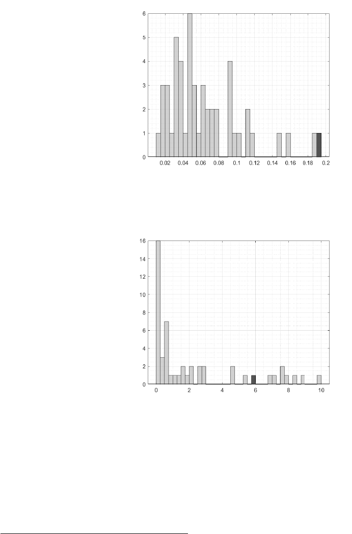
Figure 5: Post-treatment root mean square errors

Notes: Auckland appears in black.

Figure 6: Negative-error RMSE ratios

Notes: Auckland appears in black.

RMSE Ratio”, or NE-RMSE-R.

Figure 6 depicts the histogram of the ratios. Auckland is ranked ninth out of ﬁfty,

outside conventional levels of statistical signiﬁcance. While its post-intervention RMSE

is second largest, Auckland’s pre-intervention RMSE is also somewhat large, causing the

NE-RMSE-R to be ranked somewhat lower that the post intervention RMSE.

Because the ﬁnal pre-intervention observations are normalized to zero, the pre-intervention RMSE

omits the intervention year.

Figure 7: Leave-one-out robustness check

2000 2002 2004 2006 2008 2010 2012 2014 2016 2018 2020 2022

-0.8

-0.6

-0.4

-0.2

0.2

0.4

0.6

Notes: Leave-one-out replications in gray. The synthetic control for the full sample is the red dashed line.

4.4 Robustness Checks

4.4.1 Leave-One-Out

We perform the “leave one out” robustness check (Abadie et al., 2010), whereby units from

the donor pool are iteratively removed from the sample while the procedure is repeated.

This procedure examines the extent to which the synthetic control may be dependent on

any single given donor unit.

Figure 7 exhibits the full-sample synthetic control (FS-SC, given by the red dashed line)

alongside leave-one-out synthetic controls (LOO-SCs, given by the gray lines). In general,

each of the LOO-SCs follow a common trend over both the pre- and post- sample period.

This indicates that the results are not particularly sensitive to any one urban area being

included in the donor set.

There is, however, one clear case in Figure 7 where synthetic rents are slightly lower

over the post-treatment period. This corresponds to when Rotorua, which receives a weight

of almost three quarters, is omitted from the donor set.

Given that results are somewhat sensitive to the inclusion of Rotorua in the donor

set, we single out the case where Rotorua is left out. Under this speciﬁcation, Tauranga

receives a weight of 0.575, while Palmerston North receives 0.424. The latter is a large

urban area of approximately 100,000 residents, 400km south of Auckland. Table 4 in

the Appendix exhibits the matching variables, showing that population growth is now

much better matched by the synthetic unit, while the match to the proportion of renting

households is slightly worse.

The top panel of Figure 8 depicts actual and synthetic rental price indexes. The syn-

thetic control implies a 0.243 reduction in log rents, corresponding to 21.6% decrease.

Equivalently, rents would be 27.6% higher under the counterfactual of no reform (since

0.276 = 0.216/(1 − 0.216)). Auckland’s post intervention RMSE still ranks ﬁrst among

placebos, indicating that the smaller reduction is nonetheless statistically signiﬁcant when

evaluated by this measure. It’s NE-RMSE-R ranks twelfth.

As discussed in the introduction, we select this as our preferred speciﬁcation. The

inclusion of a single unit – Rotorua – in the donor set has a substantial eﬀect on estimated

policy impacts. Once it is removed from the donor set, the policy impact is somewhat

smaller in magnitude. To be conservative in our assessment, we headline these results as

our preferred empirical speciﬁcation.

4.4.2 Unrestricted Selection of Donor Units

In our baseline set of models, donor units for Auckland and “metropolitan” and “large”

urban areas are restricted. In this subsection we present results when these restrictions are

not imposed, such that donor units for Auckland comprise the other 49 urban areas in the

sample.

Rotorua, Gore and W¯anaka receive weights of 0.678, 0.204, and 0.118. Thus, the large

weight on Rotorua is similar to the baseline speciﬁcation presented in section 4.2, while

Gore and W¯anaka replace Invercargill and Tauranga. W¯anaka is a small urban area 990

km south from Auckland (as the crow ﬂies) with a population of 15,000, while Gore in

a small urban area 1150 km south of Auckland with an estimated population of 12,500.

The middle panel of Figure 8 exhibits synthetic and actual rental indexes. By 2022, log

rents in Auckland are 0.310 less than the synthetic control, corresponding to a 26.7 percent

(= 1 − e

−0.310

) decrease in rents relative to the counterfactual of no zoning reform. Thus,

under non-hierarchical selection, the decrease in rents due to the reform is estimated to

be even larger. Auckland has the second largest post-treatment RMSE. The probability

of obtaining the largest RMSE is 0.041 ( = 2/49). Meanwhile, Auckland’s NE-RMSE-R

ranks tenth

4.4.3 Population Decreases after COVID-19

According to Statistics New Zealand estimates, Auckland’s population decreased by 1.07%

between 2020 and 2022.

The ability of the synthetic control to account for the eﬀect of

a population decrease on rents in Auckland depends on whether the matching variables

Population estimates are as at June. For information on methodology, see https://datainfoplus.

stats.govt.nz/item/nz.govt.stats/951e3175-d94d-4d67-9af7-47c0a75f90d9/7. As of May 2023,

the subnational population estimates at 30 June 2021 and 2022 are both provisional. Estimates for the

year to June 2023 were released on 25 October, showing that there was a 2.8% increase in the Auckland

Region’s population over this period. This gain is more than suﬃcient to reverse the loss in population

over the previous two years.

Figure 8: Synthetic and actual rental price indexes, robustness checks

2000 2002 2004 2006 2008 2010 2012 2014 2016 2018 2020 2022

Year

-0.8

-0.6

-0.4

-0.2

0.2

0.4

0.6

Log Rent Price Index

Actual Auckland

Synthetic Auckland

2000 2002 2004 2006 2008 2010 2012 2014 2016 2018 2020 2022

Year

-0.8

-0.6

-0.4

-0.2

0.2

0.4

0.6

Log Rent Price Index

Actual Auckland

Synthetic Auckland

2000 2002 2004 2006 2008 2010 2012 2014 2016 2018 2020 2022

Year

-0.8

-0.6

-0.4

-0.2

0.2

0.4

0.6

Log Rent Price Index

Actual Auckland

Synthetic Auckland

Notes: Top: Donor with the largest weight (Rotorua) omitted from the donor set. Middle: Unrestricted

selection of donors, including medium and small urban areas. Bottom: Matching to urban areas with

population decreases between 2020 and 2022.

Figure 9: Rental prices for urban areas with population decreases between 2020 and 2022

2000 2002 2004 2006 2008 2010 2012 2014 2016 2018 2020 2022

Year

0.4

0.6

0.8

1.2

1.4

1.6

1.8

Rent Price Index (2016 = 1)

Reform

Auckland

Wellington

Dunedin

Rotorua

Invercargill

Notes: Rental price indexes for urban areas that experienced a decrease in estimated population between

2020 and 2022.

select control units that experienced similar decreases. In this regard, Auckland was not

unique among urban areas in experiencing a decline. Among the metropolitan and large

urban centers, Wellington (-0.16%), Dunedin (-1.83%), Rotorua (-0.55%), Invercargill (-

0.53%) also experienced decreases in (estimated) population. Notably, some of these urban

areas already feature in the selected donor pool for Auckland, suggesting that the set

of predictors may span the set of variables that explain the population decline. Figure

9 depicts rents of urban areas that experienced population decreases between 2020 and

2022. All except Auckland exhibit substantial appreciation from 2016 onwards, including

Dunedin, which is notable for being the urban area that experienced a larger population

exodus than Auckland. Thus, despite having a larger population exodus than Auckland,

Dunedin experienced a substantially larger increase in rents.

Although Auckland was not the only urban area to experience a population decrease, the

incidence and responses to COVID-19 may present a unique shock that disproportionately

aﬀected Auckland and that proves diﬃcult for the synthetic control to adequately model

from 2020 onwards.

We modify our empirical strategy in two diﬀerent ways to address this potential problem.

First, we end the sample in 2020, when estimated population in Auckland peaks. Second, we

re-specify the set of matching variables to comprise the decrease in population from 2020

to 2022, and a limited number of rental market characteristics. This tilts the synthetic

control procedure towards selecting urban areas that experienced a decrease in population

from 2020 onwards.

Ending the sample in 2020. By 2020, log rents in Auckland are 0.192 less than the

synthetic control, corresponding to a 17.3 percent (= 1 − e

−0.190

) decrease in rents relative

to the counterfactual of no zoning reform. Auckland has the largest post-intervention

RMSE, meaning that the probability of obtaining a RMSE that is largest is 0.02 ( = 1/50).

Auckland’s NE-RMSE-R ranks eighth.

Matching post 2020 population decreases. We set the matching variables to include

the log population change between 2020 and 2022. We also include the proportion of people

aged 18 to 22 inclusive, to account for the potential eﬀect of the border closure and interna-

tional students returning home, in 2013. Both Auckland and Dunedin, which experienced

the largest population decreases, have a large tertiary sector that serves international as

well as domestic students. We also restrict the donor pool to urban areas that experienced

a population decrease between 2020 and 2022.

Motueka, Dunedin, Rotorua, Gore, Invercargill, Dannevirke and Wellington receive

weights of 0.319, 0.267, 0.0947, 0.0946, 0.0913, 0.071 and 0.062. The model is able to

match population decrease exactly due to the few number of matching variables. The

bottom panel of Figure 8 exhibits synthetic and actual rents. Pre-intervention ﬁt of the

synthetic unit is noticeably impaired when compared to the baseline model. By 2022, log

rents in Auckland are 0.261 less than the synthetic control. This is a smaller decrease

than under the baseline model, but nonetheless implies a 22.9% (= 1 − e

−0.261

) reduction

in rents. Auckland has the eighth largest post-intervention RMSE, and the third largest

NE-RMSE-R. The probability of obtaining a ratio that is third largest is 0.06 ( = 3/50).

5 Concluding Remarks

In 2016, Auckland implemented a large-scale zoning reform that precipitated a boom in

housing construction. In this paper we adopt a synthetic control approach to evaluate the

impact of the reform on rents. Across diﬀerent speciﬁcations, the synthetic control method

indicates that, six years on, rents in Auckland would be at least 27% higher had Auckland

not pursued this reform.

The eﬀects of large-scale upzoning posited by advocates of reform should no longer be

considered to be purely theoretical. Auckland’s experience suggests that zoning reform

can stimulate housing supply and reduce housing costs. Policymakers seeking to redress

persistent housing shortages and unaﬀordability should consequently consider reforming

residential zoning codes to allow cities to build medium and high density housing.

Our ﬁndings for Auckland are, however, a medium-run evaluation of the reform, given

the six-year horizon of the study. Long-run eﬀects may depend on inter-regional migration

in response to lower housing costs, with in-migrants potentially eroding away reductions

in rents, and underscoring the need for coordinated or concurrent action across diﬀerent

cities. New Zealand’s recently-elected center-right government has pledged to repeal similar

reforms that it recently helped pass to enable medium density housing in New Zealand’s

largest cities.

Repealing this legislation will potentially increase in-migration pressures

into Auckland in response to its earlier, unilateral, reform, potentially reducing the eﬀect

of the reform on housing aﬀordability over the long term if other large cities do not (or are

not incentivised to) follow Auckland’s lead and reform their zoning codes to allow more

housing development.

We conclude by noting that housing costs in Auckland remain among the most ex-

pensive in the world, as measured by either the proportion of disposable income spent on

housing or house prices relative to incomes. This observation is not, however, evidence

against the eﬃcacy of Auckland’s reform, since it leaves the counterfactual unspeciﬁed.

The evidence presented herein indicates that housing costs would have been even more

expensive had Auckland not reformed its zoning code. Nonetheless, our ﬁndings do sug-

gest that Auckland’s reform is not a panacea, and that additional policy tools and further

reforms may be necessary to bring housing costs down to aﬀordable levels.

In December 2021, the center-left Labour and center-right National parties voted to pass the Medium

Density Residential Standard (MDRS), which requires the ﬁve largest cities in New Zealand to employ a

medium density default of three storeys and three dwellings per parcel in residential areas. To date, only

two councils (Hutt City and Upper Hutt) have operationalized the MDRS.

6 Appendix

6.1 Hedonic Imputation Index

Our sample of rental bonds consists of apartments, houses and ﬂats. Bonds with no record

of the dwelling type are omitted. We restrict the sample to private dwellings, as many

public rentals are subsidized, and this is the convention followed by Statistics New Zealand

when constructing rental price indexes. Let p

i(t),t

denote the logged weekly rent of house

i (t) sold in period t, and let X

i(t),t

be a vector of characteristics. The hedonic regression is

i(t),t

= X

′

i(t),t

+ ε

i(t),t

, (2)

where t = 1, ..., T indexes time periods (years), and i(t) = 1(t), ..., n(t) indexes the cross

sections observed in period t. We include the following observable characteristics in X

i(t),t

number of bedrooms, a dummy for apartment, a dummy for ﬂat, and locational dummies

(speciﬁcally, SA2 dummies). The vector of characteristics X

i(t),t

also includes a constant.

For each FUA, we ﬁt (2) to the cross section of rents for t = 1, ..., T , obtaining

t=1

. For each observation i(t) in period t, we use the estimated hedonic function to impute

rents in period t as ˆp

i(t),t

= X

i(t),t

′

, and t − 1 as ˆp

i(t),t−1

= X

i(t),t

′

t−1

. We then run the

following regression

ˆp

i(t),t

− ˆp

i(t),t−1

= δ

+ u

i(t),t

, t = 2, ..., T

The sequence

t=1

yields the hedonic imputation price index, where

= 0.

6.2 Additional Tables and Figures

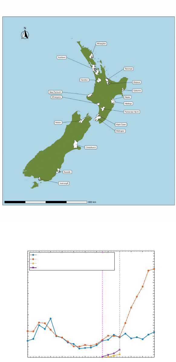
Figure 10: Metropolitan and large urban areas of New Zealand

Figure 11: New dwelling permits in Auckland by 2016 zoning change, 2000 to 2022

2000 2002 2004 2006 2008 2010 2012 2014 2016 2018 2020 2022

New dwelling permits (thousands)

Reform

Partial Reform

Non-Upzoned Residential, Business and Rural Areas

Upzoned Residential and Business Areas

PAUP-SpHA in Non-Upzoned Areas

PAUP-SpHA in Upzoned Areas

Notes: New dwelling permits in areas that were and were not upzoned in 2016 under the AUP, with permits

issued under to Special Housing Areas (SpHA) separately identiﬁed. See notes to Figure 1 for additional

details.

Table 3: Functional urban area statistics

Urban Area Population Dwellings Pers. Inc. ($) Area (km

) Prop. dev. land Dist. Auck. (km)

Auckland 1,567,038 490,695 36,000 3356.9 0.4532 -

Hamilton 209,970 70,596 33,700 1412.7 0.8217 114

Tauranga 156,666 57,690 33,300 789.9 0.3942 155

Wellington 422,427 149,820 39,700 1754.2 0.1212 493

Christchurch 482,088 177,135 35,400 2408.0 0.5797 764

Dunedin 132,006 49,533 27,400 1033.8 0.2278 1,064

Whang¯arei 86,538 31,407 29,000 1433.6 0.5402 131

Rotorua 74,028 24,795 29,100 649.2 0.5902 194

Gisborne 43,953 15,360 28,000 612.8 0.2432 350

Hastings 79,431 26,823 29,700 1160.4 0.5142 359

Napier 66,459 24,834 30,400 259.8 0.3496 348

New Plymouth 80,997 31,002 31,800 920.9 0.3967 253

Whanganui 45,747 18,249 25,400 598.1 0.3374 344

Palmerston North 96,552 34,737 32,000 978.3 0.7821 397

K¯apiti Coast 46,839 19,128 32,100 317.4 0.1705 452

Nelson 84,846 31,833 31,300 1177.2 0.1855 508

Invercargill 55,386 21,825 31,700 428.5 0.7148 1,188

Source: Authors’ calculations based on 2018 census. Notes: Only metropolitan and large urban areas are

tabulated. Dwellings are occupied dwellings. Note that Christchurch is omitted from Auckland’s donor

pool due to the eﬀect of the 2011 earthquakes on the housing stock and subsequent rebuild.

Table 4: Matched variables, Rotorua omitted from donors

Variable Auckland Synthetic Auckland Average of Donors

Dwellings per capita, 2013 0.332 0.389 0.389

Dwellings per capita, 2006 0.338 0.387 0.386

Dwellings per capita, 2001 0.343 0.386 0.385

Population growth, 2006 to 2013 0.125 0.115 0.071

Population growth, 2001 to 2006 0.091 0.084 0.033

Proportion of developable land 0.453 0.527 0.361

Personal income ($), 2013 30,200 27,926.99 27,808.35

Personal income ($), 2006 27,200 23,742.41 23,399.14

Personal income ($), 2001 21,500 17,552.28 17,549.18

Proportion of households renting, 2013 0.388 0.347 0.333

Proportion of household renting, 2006 0.363 0.332 0.314

Proportion of income spent on rent, 2013 0.262 0.252 0.251

Proportion of income spent on rent, 2006 0.244 0.227 0.229

Notes: Matching variables also include rent indexes, 2000 to 2016. These are not tabulated for the sake of

brevity. Population growth is log diﬀerence of estimated population. Proportion of income spent on rent

is based on pre-tax income for renting households.

References

Abadie, A. (2021): “Using Synthetic Controls: Feasibility, Data Requirements, and

Methodological Aspects,” Journal of Economic Literature, 59. 4, 12, 13, 16

Abadie, A., A. Diamond, and J. Hainmueller (2010): “Synthetic control methods for

comparative case studies: Estimating the eﬀect of California’s Tobacco control program,”

Journal of the American Statistical Association, 105, 493–505. 4, 11, 12, 16, 18

Abadie, A. and J. Gardeazabal (2003): “American Economic Association The Eco-

nomic Costs of Conﬂict: A Case Study of the Basque Country,” The American Economic

Review, 93, 113–132. 11, 12

Been, V. (2018): “City NIMBYs,” Journal of Land Use and Environmental Law, 33,

217–250. 2

Bentley, A. (2022): “Rentals for Housing: A Property Fixed-Eﬀects Estimator of Inﬂa-

tion from Administrative Data,” Journal of Oﬃcial Statistics, 38, 187–211. 8

Cheung, K. S., P. Monkkonen, and C. Y. Yiu (2023): “The heterogeneous impacts

of widespread upzoning: Lessons from Auckland, New Zealand,” Urban Studies. 3

Clapp, J. M. and C. Giaccotto (1992): “Estimating price indices for residential

property: A comparison of repeat sales and assessed value methods,” Journal of the

American Statistical Association, 87, 300–306. 8

Dong, H. (2021): “Exploring the Impacts of Zoning and Upzoning on Housing Develop-

ment: A Quasi-experimental Analysis at the Parcel Level,” Journal of Planning Educa-

tion and Research, 00, 1–13. 3

Eurostat (2013): Handbook on Residential Property Prices (RPPIs). 8

Freeman, L. and J. Schuetz (2017): “Producing Aﬀordable Housing in Rising Markets:

What Works?” Cityscape, 19. 2

Freemark, Y. (2020): “Upzoning Chicago: Impacts of a Zoning Reform on Property

Values and Housing Construction,” Urban Aﬀairs Review, 56, 758–789. 3

Glaeser, E. L. and J. Gyourko (2003): “Building restrictions and housing availabil-

ity,” Economic Policy Review, 21–39. 2

Greenaway-McGrevy, R. (2023a): “Can Zoning Reform Increase Housing Construc-

tion? Evidence from Auckland,” Economic Policy Centre Working Paper 017. 2, 6,

——— (2023b): “Evaluating the Long-Run Eﬀects of Zoning Reform on Urban Develop-

ment,” Economic Policy Center Working Paper 013. 3

Greenaway-McGrevy, R. and J. A. Jones (2023): “Can zoning reform change urban

development patterns? Evidence from Auckland,” Economic Policy Centre Working

Paper 012. 2, 5

Greenaway-McGrevy, R., G. Pacheco, and K. Sorensen (2021): “The eﬀect of

upzoning on house prices and redevelopment premiums in Auckland, New Zealand,”

Urban Studies, 58, 959–976. 3

Greenaway-McGrevy, R. and P. Phillips (2023): “The Impact of Upzoning on

Housing Construction in Auckland,” The Jounral of Urban Economics, 136, 103555. 2

Greenaway-McGrevy, R. and P. C. B. Phillips (2021): “House prices and aﬀord-

ability,” New Zealand Economic Papers, 55, 1–6. 7

Gyourko, J. and R. Molloy (2015): “Regulation and Housing Supply,” Handbook of

Regional and Urban Economics, 5, 1289–1337. 2

Hamilton, E. (2021): “Land Use Regulation and Housing Aﬀordability,” in Regulation

and Economic Opportunity, ed. by A. Hoﬀer and T. Nesbit, Center for Growth and

Opportunity at Utah State University, 186–202. 2

Hansen, N. (2016): “The CMA Evolution Strategy: A Tutorial,” arXiv preprint

arXiv:1604.00772. 12

Li, Z., X. Lin, Q. Zhang, and H. Liu (2020): “Evolution strategies for continuous

optimization: A survey of the state-of-the-art,” Swarm and Evolutionary Computation,

56. 12

Pakes, A. (2003): “A Reconsideration of Hedonic Price Indexes with an Application to

PC’s,” American Economic Revieweview, 93, 1578–1596. 8

Rodr

ıguez-Pose, A. and M. Storper (2020): “Housing, urban growth and inequali-

ties: The limits to deregulation and upzoning in reducing economic and spatial inequal-

ity,” Urban Studies, 57, 223–248. 3

Saiz, A. (2010): “The Geographic Determinants of Housing Supply,” The Quarterly Jour-

nal of Economics, 125, 1253–1297. 11

——— (2023): “The Global Housing Aﬀordability Crisis: Policy Options and Strategies,”

MIT Center for Real Estate Research Paper No. 23/01. 2

Schill, M. H. (2005): “Regulations and Housing Development: What We Know,”

Cityscape, 8, 5–19. 2

Silver, M. and S. Heravi (2007): “The diﬀerence between hedonic imputation indexes

and time dummy hedonic indexes,” Journal of Business and Economic Statistics, 25,

239–246. 8

Stacy, C., C. Davis, Y. S. Freemark, L. Lo, G. MacDonald, V. Zheng, and

R. Pendall (2023): “Land-use reforms and housing costs: Does allowing for increased

density lead to greater aﬀordability?” Urban Studies, 1–22. 3

Wetzstein, S. (2017): “The global urban housing aﬀordability crisis,” Urban Studies, 54,

3159–3177. 2